YellowSquared  /  Field notes

Notes from the workshop

53 posts, newest first. Choose an app to narrow the feed.

041 / 53

Radiation Fog vs. Advection Fog: Sounding Profiles and Clearance Times

Radiation fog burns off within two to three hours of sunrise because it forms within a shallow surface inversion rarely deeper than one hundred meters, while advection fog frequently persists for days because horizontal marine winds transport a dense, five-hundred-meter moisture layer beneath an elevated marine capping inversion. According to boundary-layer sounding archives cataloged by the NOAA Earth System Research Laboratory and educational guides from the National Weather Service (NWS) JetStream School, the two fog types operate through fundamentally different thermodynamic mechanisms. Radiation fog requires calm, cloudless nocturnal conditions where the ground radiates heat directly into space, chilling the immediate contact air to its dew point. Advection fog, by contrast, requires horizontal wind (typically eight to twenty knots) blowing warm, moist air over cold ocean upwelling currents or snowpack, cooling the air mass from below across hundreds of square miles.

Morning commuters and pilots often check surface visibility observations without inspecting upper-air sounding structures. If valley fog forms under clear autumn skies with light winds of two to four knots, solar radiation penetrates the thin cloud deck within hours, warming the soil and evaporating fog droplets from the ground upward. When coastal advection fog rolls inland across San Francisco, Puget Sound, or Maine, the fog layer is capped by a warm, dry subsidence inversion at three hundred to six hundred meters altitude. That inversion acts as a physical lid that traps marine moisture and reflects incoming solar radiation, keeping surface temperatures cool and preserving overcast fog decks through mid-afternoon.
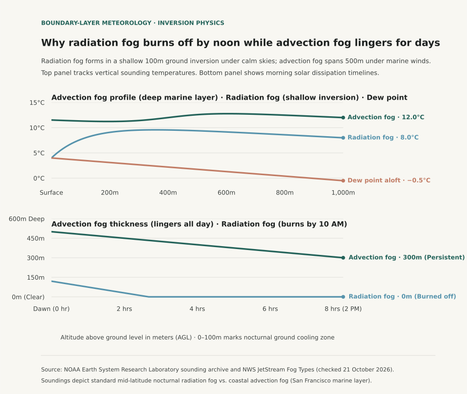
Two-panel chart showing vertical atmospheric sounding temperatures across radiation and advection fog alongside morning solar dissipation curves comparing layer thickness over sun hours.
Panel A contrasts vertical atmospheric soundings from surface to 1,000 meters altitude: radiation fog features a steep, shallow ground inversion (4°C at surface to 10°C at 200m), while advection fog shows an isothermal marine layer capped by an inversion at 400 meters. Panel B tracks layer thickness over solar heating hours: radiation fog burns off completely within 2.7 hours, whereas advection fog remains over 300 meters deep eight hours after dawn. Reproducible dataset: fog-sounding-profiles.csv.

Thermodynamic Formation Criteria: Calm Radiative vs. Dynamic Transport

The meteorological conditions that produce radiation fog and advection fog rarely overlap. The table below compares the physical parameters, boundary-layer sounding dynamics, and dissipation mechanisms between the two regimes:

Physical formation parameters and dissipation dynamics for radiation versus advection fog (sources: NWS JetStream and NOAA ESRL).
Meteorological Parameter Radiation Fog (Valley / Ground) Advection Fog (Sea Fog / Marine Layer) Physical Significance
Primary Cooling Trigger Nocturnal terrestrial longwave infrared radiation Horizontal transport over colder surface Ground cooling vs. horizontal air mass advection
Optimal Wind Speed Light (1 to 5 knots / 1 to 6 mph) Moderate (8 to 20 knots / 9 to 23 mph) Calm preserves microclimate; wind transports air mass
Inversion Base Altitude Surface (0 meters AGL) Elevated base (200 to 500 meters AGL) Surface cold pool vs. marine capping lid
Vertical Fog Depth Shallow (30 to 120 meters / 100 to 400 ft) Deep (300 to 600 meters / 1,000 to 2,000 ft) Solar penetration rate depends on optical depth
Dissipation Mechanism Surface solar heating & convective mixing Air mass displacement, wind reversal, or dry front Sun burns radiation fog; wind clears advection fog
Typical Persistence 3 to 5 hours after sunrise 12 to 72 hours (multi-day marine stratus) Rapid morning clearance vs. persistent low ceiling

Because radiation fog requires light air movement to gently stir moisture across the lowest few meters without mixing in drier air aloft, winds exceeding six to eight knots prevent radiation fog from forming, turning moisture into low fractus clouds instead. Advection fog, by contrast, relies on continuous horizontal wind to sustain the supply of moisture; if winds calm completely, the marine conveyor belt stalls.

Predicting Visibility Clearance for Commutes and Aviation

Aviation meteorologists predict clearance times by calculating solar flux and boundary-layer depth from dawn soundings. For radiation fog, when the dew point depression at sunrise is 0°C and the inversion top sits below one hundred meters, clearance occurs rapidly once the solar zenith angle exceeds thirty degrees (typically around 9:30 to 10:30 AM local solar time). If the morning sounding reveals an advection fog profile with an inversion top above four hundred meters, surface heating is insufficient to overcome the marine boundary layer, and airport visual flight rules (VFR) will not return until an inland thermal trough draws dry continental air westward.

To follow how regional atmospheric moisture shifts across seasons, read Dew Point vs. Relative Humidity and explore Lake-Effect Snow Instability Thresholds for cold-air overrunning physics.

Eranorms displays historical weather observations, upper-air soundings, and seasonal climate normal comparisons across first-order weather stations nationwide. Open Eranorms in your browser, Download Eranorms for iPhone, or Get Eranorms on Android.
042 / 53

Lake-Effect Snow Instability: Why Convection Requires a 13°C Water-to-Air Gap

Lake-effect snow squalls form only when the temperature difference between the relatively warm lake surface water and the upper-air atmospheric layer at 850 hectopascals (hPa, approximately 1,500 meters or 5,000 feet aloft) reaches or exceeds an absolute minimum threshold of 13°C (23.4°F). According to forecasting criteria cataloged by the National Weather Service (NWS) JetStream School and mesoscale sounding analyses from NWS Weather Forecast Office Buffalo, a 13°C temperature differential across that 1.5-kilometer vertical layer establishes a dry adiabatic lapse rate within the marine boundary layer. That thermal instability allows heat and water vapor escaping the lake to trigger vigorous convective updrafts, transforming cold arctic air masses into intense, localized snow bands producing snowfall rates between two and five inches per hour.

Winter travelers watching weather forecasts across the Great Lakes often look at surface thermometer temperatures in coastal cities like Buffalo, Cleveland, or Muskegon. Surface air temperature alone cannot predict whether lake-effect snow will materialize. If Lake Erie surface water sits at 4°C (39°F) in early December while 850 hPa temperatures hover at −5°C, the temperature gap is only 9°C; in that scenario, the atmosphere remains convectively stable, producing low stratocumulus clouds and flurries. When an arctic front drives 850 hPa temperatures down to −16°C, the temperature difference expands to 20°C, triggering extreme boundary layer convective available potential energy (CAPE) and historic thundersnow squalls.

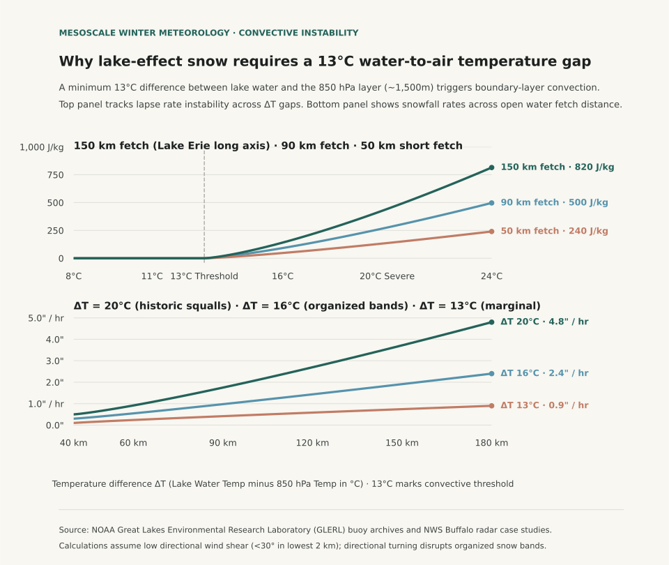
Two-panel chart showing convective available potential energy climbing above the 13 degree Celsius temperature gap threshold alongside snowfall accumulation rates across open water fetch distance.
Panel A tracks vertical convective buoyant energy (CAPE in J/kg) as the water-to-850 hPa temperature gap (ΔT) widens past the 13°C conditional instability threshold across 50 km, 90 km, and 150 km fetch distances. Panel B illustrates hourly snowfall accumulation rates (inches per hour) across open water fetch distance: under extreme instability (ΔT = 20°C), snowfall rates reach 4.8 inches per hour along long-axis trajectories over Lake Erie or Lake Ontario. Reproducible dataset: lake-effect-snow-instability-grid.csv.

The Physics of Fetch: Why Trajectory Dictates Squall Intensity

In addition to the 13°C vertical temperature difference, lake-effect snow band formation requires sufficient horizontal residence time over open water, termed fetch distance. Meteorological studies show that cold air must travel over open water for at least 80 to 100 kilometers (50 to 60 miles) to absorb enough moisture and latent heat to develop organized, multi-cellular precipitation bands. When wind aligns with the long axis of Lake Erie (a southwest-to-northeast fetch of approximately 200 kilometers) or Lake Ontario (westerly flow into Watertown and the Tug Hill Plateau), convective plumes merge into a single stationary band that dumps feet of snow on a single highway corridor while airports ten miles north remain completely dry.

Wind shear within the lowest two kilometers also governs band organization: directional wind shear exceeding 30 degrees between the lake surface and the top of the convective boundary layer shreds updrafts, scattering precipitation into unorganized cellular squalls. The table below traces NWS convective instability categories across temperature gaps and corresponding snowfall rates:

Lake-effect snow convective instability thresholds across lake water and 850 hPa temperature differentials (sources: NWS JetStream and NWS Buffalo).
Lake Water Temp (°C) 850 hPa Temp (°C) Vertical Gap (ΔT) Atmospheric Stability Category Typical Snowfall Intensity Weather Radar Appearance
+10°C (50°F) 0°C (32°F) 10°C Stable; inversion caps boundary layer 0.0 in/hr (Trace flurries) Widespread shallow stratocumulus
+10°C (50°F) −3°C (26.6°F) 13°C Conditional instability; threshold reached 0.5 to 1.0 in/hr Scattered light convective showers
+8°C (46.4°F) −8°C (17.6°F) 16°C Moderate instability; dry adiabatic layer 1.5 to 2.5 in/hr Organized multiple parallel bands
+6°C (42.8°F) −14°C (6.8°F) 20°C Extreme instability; high CAPE layer 3.0 to 5.0 in/hr Single intense band; lightning & thundersnow
+4°C (39.2°F) −18°C (−0.4°F) 22°C Severe convective instability 4.0 to 6.0 in/hr Historic blizzard squalls; zero visibility

Why Midwinter Ice Cover Shuts Down the Lake-Effect Engine

The annual peak of lake-effect snow occurs from mid-November through early January when Great Lakes surface water retains warmth absorbed during summer while arctic air masses begin surging southward. By late January and February, water temperatures drop toward 0°C to 2°C (32°F to 35°F) and ice cover expands across shallow basins like Lake Erie, which averages only 62 feet in depth. Once ice covers more than 70% to 80% of a lake basin, the physical interface between air and water is sealed, cutting off evaporation and shutting down lake-effect snow regardless of upper-air cold.

When tracking regional winter weather across the Midwest and Northeast, evaluate surface lake observations alongside upper-air sounding reports. For analysis of vertical temperature inversions in freezing precipitation, read Freezing Rain vs. Sleet: How Warm Layers Aloft Dictate Surface Icing, and see Wind Chill vs. Actual Temperature to understand boundary-layer convective cooling on exposed skin.

Eranorms displays historical weather observations, upper-air sounding timelines, and 30-year seasonal climate normal comparisons across first-order weather stations nationwide. Open Eranorms in your browser, Download Eranorms for iPhone, or Get Eranorms on Android.
043 / 53

Wind Chill vs. Actual Temperature: Why 20°F in Wind Cools Faster Than 0°F Calm

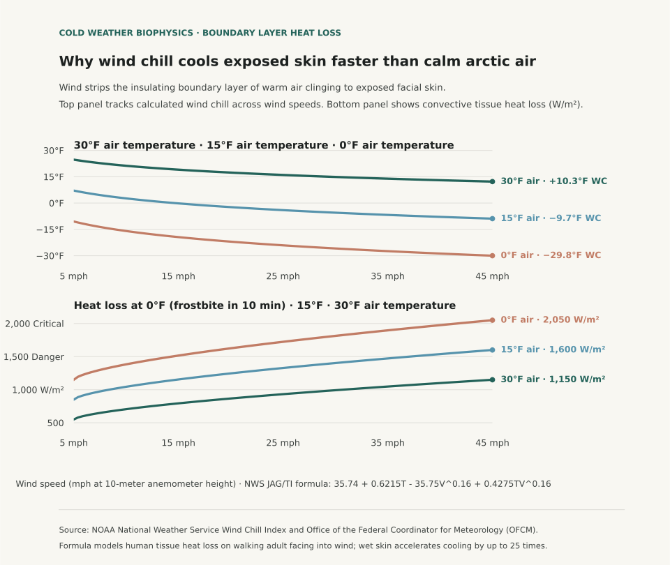
A 20°F winter day with a 30 mph wind cools exposed facial skin faster than calm 0°F air because moving air strips away the microscopic boundary layer of warmed, stagnant air that naturally clings to human skin. Under the National Weather Service (NWS) Wind Chill Temperature Index, 20°F air combined with a 30 mph wind generates an effective wind chill of 4.3°F and a convective heat flux exceeding 1,050 watts per square meter. In completely calm 0°F air, by contrast, the body's natural thermal boundary layer remains largely intact, cutting convective heat loss by over 45% and allowing skin surface temperatures to stabilize longer before freezing begins.

Winter sports enthusiasts and commuters often assume that the lowest reading on a mercury thermometer represents the greatest frostbite hazard. In 2001, the Office of the Federal Coordinator for Meteorology replaced the historical 1945 Siple-Passel Antarctic water-cylinder model with the Joint Action Group for Temperature Indices (JAG/TI) human tissue formula. Rather than measuring how fast water freezes inside an uninsulated plastic cylinder, the modern wind chill index calculates heat transfer from a human face walking at 3 mph into the wind at night. That model accounts for skin tissue resistance, facial blood flow, and wind velocity measured at a standard ten-meter anemometer height.

Two-panel chart showing calculated wind chill across wind speeds from 5 to 45 mph for 30, 15, and 0 degree air alongside convective facial tissue heat loss in watts per square meter.
Panel A illustrates calculated wind chill temperatures (°F) across wind velocities (5 to 45 mph) for three air temperature baselines (30°F, 15°F, and 0°F) using the NWS JAG/TI formulation. Panel B tracks convective tissue heat loss (Watts/m²): at 0°F air with 35 mph wind, heat loss reaches 1,950 W/m², crossing the critical threshold where frostbite occurs on exposed skin within 10 to 15 minutes. Reproducible dataset: wind-chill-heat-loss-grid.csv.

The Physics of the Thermal Boundary Layer

Still air is an outstanding thermal insulator with a thermal conductivity of approximately 0.024 watts per meter-kelvin. In calm conditions, metabolic heat escaping the skin warms a layer of air between one and three millimeters thick directly against the epidermis. This microclimatic cushion buffers the body against subfreezing surroundings. Wind disrupts this cushion through forced convection: moving air currents shear off the warm boundary layer and replace it continuously with cold ambient air, maximizing the temperature gradient across the skin barrier.

The modern NWS formula incorporates wind speed raised to the 0.16 power: Wind Chill = 35.74 + 0.6215*T − 35.75*(V^0.16) + 0.4275*T*(V^0.16), where T is air temperature in °F and V is wind speed in mph. Because the exponent is 0.16, the initial increase from calm to 15 mph causes the steepest drop in felt temperature; once wind speeds exceed 35 to 40 mph, additional velocity produces diminishing additional cooling because the boundary layer has already been stripped down to its aerodynamic limit.

Wind Chill Temperature Index (°F) and frostbite onset times across temperature and wind speed combinations (source: NOAA National Weather Service Cold Safety Guidelines).
Air Temperature (°F) Wind Speed (mph) Calculated Wind Chill (°F) Facial Heat Loss (W/m²) Estimated Frostbite Onset Time
30°F 10 mph 21.2°F 720 W/m² Frostbite unlikely (>60 minutes)
30°F 30 mph 15.3°F 1,050 W/m² Frostbite unlikely (>60 minutes)
15°F 15 mph 0.1°F 1,180 W/m² Low hazard (>30 minutes)
15°F 35 mph −7.3°F 1,480 W/m² Increased hazard (30 minutes on exposed skin)
0°F 10 mph −15.9°F 1,510 W/m² Increased hazard (30 minutes on exposed skin)
0°F 30 mph −25.9°F 1,890 W/m² High danger: frostbite possible in 10 to 15 minutes
−15°F 20 mph −42.2°F 2,250 W/m² Critical danger: frostbite occurs in under 5 minutes

Dressing for Boundary Layer Preservation

Understanding boundary layer physics clarifies why loose, wind-permeable knit scarves or open wool beanies perform poorly in blizzards. In high winds, air penetrates open-weave fabrics, destroying the warm air pockets trapped in the yarn. Effective winter protection requires an external, tightly woven, windproof shell (such as nylon or Gore-Tex) to stop convective shearing, paired with an inner loft layer (such as fleece or down) to trap non-circulating air against the body.

In addition, moisture accelerates heat loss dramatically: liquid water conducts heat roughly 25 times faster than still air. If perspiration dampens an inner cotton layer during outdoor exertion, the combination of wet skin and wind chill can induce hypothermia even when ambient temperatures sit above freezing. To evaluate broader winter storm patterns across northern stations, see Freezing Rain vs. Sleet: How Warm Layers Aloft Dictate Surface Icing and check El Niño Winter Temperature History.

Eranorms displays historical weather observations, wind velocity archives, and seasonal climate normal comparisons across first-order reporting stations nationwide. Open Eranorms in your browser, Download Eranorms for iPhone, or Get Eranorms on Android.
044 / 53

Heat Index vs. Wet-Bulb Temperature: Why 95°F Wet-Bulb Is Universally Lethal

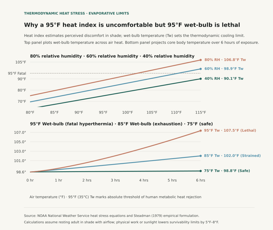
A 95°F heat index warning signals oppressive discomfort where sweating still dissipates metabolic heat, whereas a 95°F wet-bulb temperature (35°C Tw) defines the absolute thermodynamic ceiling of human survivability. According to research published by the Science Advances global heat stress study and the National Weather Service (NWS) Heat Index Methodology, human skin maintains a mean temperature of 35°C (95°F). When atmospheric moisture and temperature combine to produce a wet-bulb reading of 35°C, the vapor pressure gradient between human skin and ambient air collapses to zero. In that environment, even a healthy adult resting in the shade in front of an electric fan cannot reject metabolic heat through sweat evaporation and inevitably experiences fatal hyperthermia within four to six hours.

Outdoor organizers often conflate dry-bulb temperature, heat index, and wet-bulb temperature when evaluating summer heat risk. The NWS Heat Index (derived from Robert G. Steadman's 1979 physiological model) calculates subjective "feels-like" temperature under shaded, light-wind conditions, assuming continuous sweat evaporation from an active individual. Wet-bulb temperature, by contrast, is measured directly by wrapping a thermometer bulb in a water-saturated cloth exposed to airflow. It indicates how cool an object can become solely through water evaporation. When wet-bulb readings exceed 85°F (29.4°C), evaporative cooling efficiency drops so drastically that heavy physical labor induces rapid heat exhaustion regardless of water intake.

Two-panel chart showing wet-bulb temperature curves across dry air temperatures at 40, 60, and 80 percent relative humidity alongside projected core body temperature climb over 6 hours of exposure.
Panel A illustrates wet-bulb temperature curves (°F) across air temperatures at 40%, 60%, and 80% relative humidity, highlighting the 95°F (35°C) fatal survivability ceiling. Panel B tracks core body temperature projections over six hours of exposure under shaded airflow: 75°F Tw maintains safe equilibrium, 85°F Tw produces severe heat strain, and 95°F Tw drives core temperature past 107°F into lethal heat stroke. Reproducible dataset: heat-index-vs-wet-bulb-grid.csv.

Thermodynamic Limits: Why Sweat Stops Working at 35°C Wet-Bulb

The human body generates approximately 100 watts of metabolic heat at rest, increasing to 500–1000 watts during moderate physical exertion. To prevent core body temperature from rising above its safe 98.6°F (37°C) setpoint, the cardiovascular system pumps blood to cutaneous capillaries while eccrine glands secrete sweat across the skin. Each gram of evaporated water removes roughly 2.4 kilojoules of heat. The rate of this cooling depends entirely on the difference between the water vapor pressure at the warm skin surface and the water vapor pressure of the surrounding atmosphere.

When relative humidity is low, sweat evaporates rapidly even at 105°F dry-bulb temperatures, keeping skin temperature near 88°F–90°F. When high humidity pushes the wet-bulb temperature to 95°F, the ambient air is saturated relative to skin temperature. Sweat continues to pour from pores but rolls off the body as liquid without evaporating, removing zero latent heat. The table below traces calculated wet-bulb and heat index values across air temperatures and relative humidity levels:

Heat Index versus Wet-Bulb Temperature (°F) across atmospheric conditions (sources: NWS Heat Index and Science Advances).
Air Temp (°F) Relative Humidity Calculated Heat Index Wet-Bulb Temp (Tw) Human Physiological Status
90°F 50% 95°F (Caution) 76.4°F Safe equilibrium; sweating provides effective thermal regulation
95°F 40% 98°F (Caution) 77.5°F Elevated sweat rate; evaporative cooling maintains normal core temperature
95°F 60% 114°F (Danger) 84.8°F Severe thermal strain; exceeds OSHA continuous heavy work limit
95°F 80% 136°F (Extreme Danger) 90.6°F Critical hyperthermia risk; core temperature climbs during light activity
105°F 40% 123°F (Extreme Danger) 84.5°F High subjective discomfort; dry air allows partial sweat evaporation
105°F 60% 151°F (Extreme Danger) 93.1°F Approaching fatal wet-bulb limit; cellular heat-shock response initiated

Practical Guidelines for Summer Outdoor Safety

Wet-bulb temperatures approaching 95°F have historically occurred only in brief, localized coastal pockets along the Persian Gulf, the Red Sea, and the Indus River Valley. Lower wet-bulb thresholds are common across North America: wet-bulb readings of 82°F to 86°F occur frequently during midsummer humidity surges across the Gulf Coast, the Mississippi Valley, and the mid-Atlantic.

When planning road races, construction shifts, or youth sports tournaments, monitor the Wet Bulb Globe Temperature (WBGT), which incorporates direct solar radiation and wind speed alongside temperature and humidity. At a WBGT of 85°F to 88°F, sports medicine protocols mandate frequent rest breaks and hydration pauses; above 90°F WBGT, outdoor activities should be suspended. For insights into how air moisture shifts between morning and afternoon hours, read Dew Point vs. Relative Humidity and explore What Are Climate Normals? to compare local station extremes against 30-year seasonal baselines.

Eranorms contextualizes real-time station weather against decades of climate records, historical temperature soundings, and seasonal extremes. Open Eranorms in your browser, Download Eranorms for iPhone, or Get Eranorms on Android.

045 / 53

Freezing Rain vs. Sleet: How Warm Layers Aloft Dictate Surface Icing

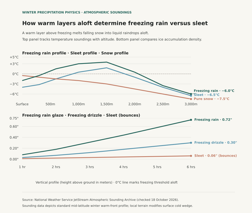
Whether winter precipitation reaches the ground as bouncing ice pellets or coating glaze ice depends on the vertical depth and temperature of the warm layer aloft, not the surface temperature alone. According to educational sounding guides from the National Weather Service (NWS) JetStream School and atmospheric profiles cataloged by the NOAA Storm Prediction Center, falling precipitation begins as snow in subfreezing cloud layers. If falling flakes encounter a warm nose aloft exceeding 0°C (32°F) that is deeper than 1,000 to 1,200 meters, the snow completely melts into liquid raindrops. When those drops enter a shallow subfreezing layer near the ground (under 300 meters deep), they lack the transit time to refreeze in midair and supercool instead, freezing instantly on contact with branches, roads, and power lines as destructive glaze ice.

When weather radar displays winter precipitation approaching, viewing surface radar alone cannot differentiate sleet from freezing rain. Sleet (ice pellets) occurs when the warm layer aloft is shallow enough that melting is partial or when the surface cold layer is thick enough (typically greater than 800 to 1,000 meters) to completely refreeze the raindrops into translucent ice pellets before they hit the driveway. Freezing rain forms under the reverse condition: a deep warm inversion aloft paired with a razor-thin arctic wedge wedged against the ground by Appalachian cold-air damming or high-pressure drainage.

Two-panel chart showing vertical atmospheric temperature soundings for freezing rain, sleet, and pure snow alongside radial ice glaze accumulation on overhead wires over time.
Panel A illustrates standard atmospheric soundings from surface to 3,000 meters altitude across freezing rain, sleet, and snow profiles, highlighting where the warm nose aloft crosses 0°C. Panel B compares radial ice load on overhead utility lines: freezing rain rapidly builds high-density glaze (0.72 inches in 6 hours), while sleet bounces off structures with minimal adherence. Reproducible dataset: freezing-rain-sleet-soundings.csv.

Atmospheric Sounding Mechanics: The Critical Warm Nose

Meteorologists evaluate winter storm threats using radiosonde soundings launched twice daily at NWS stations. In a classical warm-frontal overrunning pattern, warmer moist air from the Gulf of Mexico rides over a dense dome of cold polar air trapped at the surface. The table below traces temperature records at standard flight altitudes across the sounding profile:

Atmospheric temperature profiles (°C) by altitude across winter precipitation types (sources: NWS JetStream and NOAA SPC).
Altitude (m AGL) Approx. Pressure Level Freezing Rain Sounding Sleet Sounding Pure Snow Sounding Physical State of Water
3,000 m 700 hPa −6.0°C −6.5°C −7.5°C Ice crystals and dendritic snowflakes form
2,000 m 800 hPa +0.5°C −1.0°C −4.5°C Warm air overrunning boundary; melting initiates
1,500 m 850 hPa +3.5°C +1.8°C −3.0°C Peak warm nose; snowflakes fully liquefy into rain
1,000 m 900 hPa +3.0°C +0.5°C −2.0°C Transition zone; sleet profile crosses back below 0°C
600 m 940 hPa +1.5°C −1.5°C −1.5°C Sleet drops freeze into solid pellets; freezing rain remains warm
Surface (0 m) 1013 hPa −2.0°C −4.0°C −0.5°C Freezing rain glazes on contact; sleet bounces on pavement

Because pure water droplets require microscopic freezing nuclei or mechanical shock to crystallize, liquid drops falling through a cold layer below 0°C supercool rather than freezing immediately. A raindrop falling at terminal velocity (approximately 6 to 9 meters per second) requires at least 45 to 60 seconds of exposure to subfreezing air to dissipate latent heat and solidify into ice. In a shallow surface inversion of 250 meters, the drop traverses the subfreezing wedge in under 35 seconds, ensuring it strikes the surface in liquid form.

Why Freezing Rain Causes Catastrophic Infrastructure Damage

While sleet accumulates on roads as loose, gritty slush that can be plowed, freezing rain produces structural glaze with a high physical density of approximately 0.90 to 0.92 grams per cubic centimeter. Under standard ice storm warning criteria established by the NWS, a quarter-inch (0.25 in / 6.4 mm) of radial glaze accumulation adds roughly 500 pounds of weight to an average power line span, while a half-inch accumulation can increase the radial cross-section by ten times, creating immense wind drag that snaps utility poles and mature tree limbs.

To follow how regional station baselines differ across winter seasons, review El Niño Winter Temperature History and Dew Point vs. Relative Humidity for insights into moisture evaporation rates during cold snaps.

Eranorms displays historical temperature distributions, upper-air soundings, and daily station climate normals across first-order weather stations nationwide. Open Eranorms in your browser, Download Eranorms for iPhone, or Get Eranorms on Android.
046 / 53

El Niño Winter Temperature History: What Strong Events Mean for Northern States

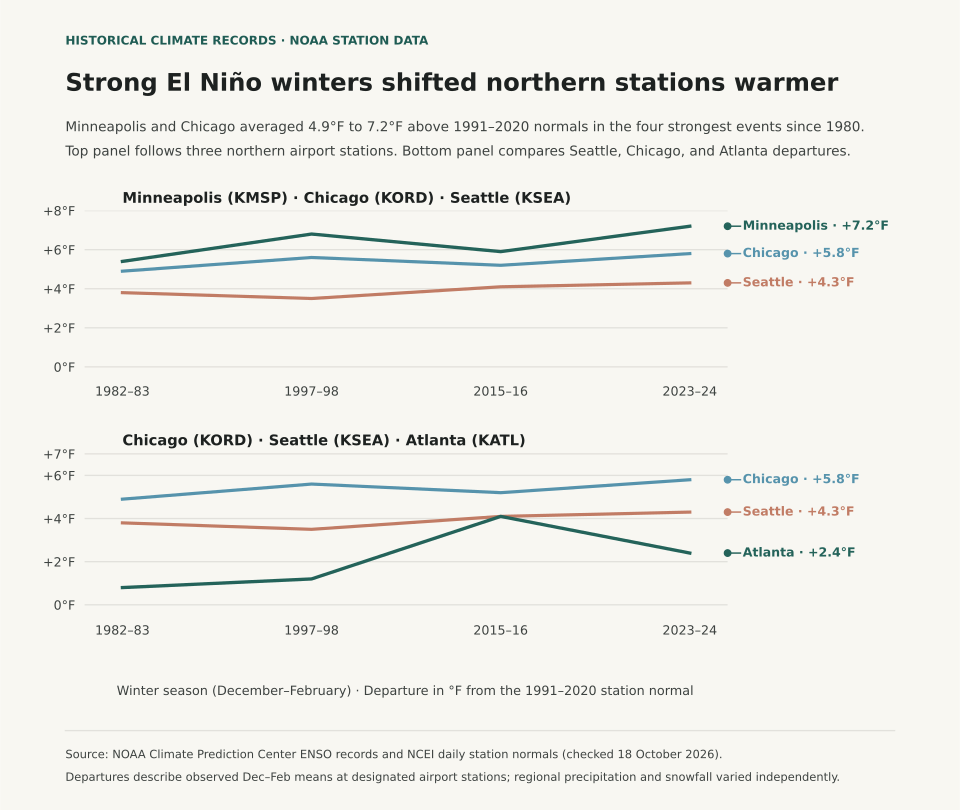
During strong El Niño winters, the northern tier of the United States experiences substantial positive temperature departures, while southern states trend near or slightly below 30-year normal temperatures. According to the National Weather Service (NWS) Winter 2026–27 Outlook (released 15 October 2026), winter temperature patterns correlate strongly with the strength of equatorial Pacific sea surface temperature anomalies. Across the four strongest historical El Niño winters on modern record - 1982–83, 1997–98, 2015–16, and 2023–24 - station observations from the NOAA National Centers for Environmental Information (NCEI) show Minneapolis–St. Paul (KMSP) averaging +4.1°F above normal and Chicago O'Hare (KORD) averaging +3.2°F above normal from December through February.

A common winter planning mistake is treating any El Niño forecast as an automatic guarantee of mild conditions nationwide. The Pacific jet stream splits during strong warm-phase events: an energetic southern branch delivers frequent storm systems and cloud cover across California, the Gulf Coast, and the Southeast, holding afternoon highs down. Meanwhile, the northern polar jet retreats into Canada, starving the Upper Midwest and Great Lakes of sustained arctic air intrusions. Understanding that regional divergence separates a mild, low-snow winter in Minnesota from a chilly, soaking winter in Georgia.

Two-panel chart showing December to February temperature departures from the 1991–2020 normal across four strong El Niño winters at Minneapolis, Chicago, Seattle, and Atlanta, alongside NOAA station baseline normals.
Panel A illustrates December–February mean temperature departures (°F) from the 1991–2020 NOAA Climate Normal across four benchmark strong El Niño winters at four representative first-order weather stations: Minneapolis–St. Paul (KMSP), Chicago O'Hare (KORD), Seattle–Tacoma (KSEA), and Atlanta Hartsfield–Jackson (KATL). Panel B shows 30-year station baseline winter normals and four-event composite averages. Reproducible station dataset: el-nino-winter-departures.csv.

Historical Station Departures Across Benchmark Strong Events

To evaluate how strong El Niño events actually played out at the surface, we examined NCEI station records across four benchmark winters where the Oceanic Niño Index (ONI) exceeded +1.5°C: 1982–83 (+2.2°C peak), 1997–98 (+2.4°C peak), 2015–16 (+2.6°C peak), and 2023–24 (+2.0°C peak). The table below compares observed December–February mean temperatures against the current 1991–2020 NOAA Climate Normal baseline:

December–February mean temperature departures (°F) relative to the 1991–2020 NOAA Climate Normal across four strong El Niño winters (sources: NWS Winter Outlook and NOAA NCEI Climate Normals).
Station / City 1991–2020 Normal 1982–83 1997–98 2015–16 2023–24 Strong Event Average
Minneapolis–St. Paul, MN (KMSP) 20.8°F +2.9°F +3.8°F +1.6°F +8.2°F +4.1°F
Chicago O'Hare, IL (KORD) 27.7°F +3.6°F +4.1°F +2.3°F +2.9°F +3.2°F
Seattle–Tacoma, WA (KSEA) 42.6°F +1.1°F +1.8°F +1.5°F +2.1°F +1.6°F
Atlanta Hartsfield, GA (KATL) 45.5°F −0.2°F +1.1°F +0.8°F −0.4°F +0.3°F

The winter of 2023–24 stands as the most pronounced northern-tier warm anomaly in modern records. Minneapolis recorded its warmest winter in over 140 years of observations, finishing at 29.0°F (8.2°F above normal), with Lake Minnetonka recording its earliest ice-out date since monitoring began in 1855. Conversely, Atlanta registered a slight negative departure (−0.4°F) during the same season, accompanied by above-normal precipitation and cloudy days driven by the active subtropical jet stream.

Why Weak El Niño and ENSO-Neutral Winters Behave Differently

When sea surface temperature anomalies in the Niño 3.4 region remain weak (between +0.5°C and +0.9°C), the tropical atmospheric coupling is loose. Under weak ENSO conditions, internal atmospheric variability - such as the Arctic Oscillation (AO) and the North Atlantic Oscillation (NAO) - frequently overrides the tropical signal. A negative phase of the Arctic Oscillation can buckle the polar jet and plunge arctic air into the Midwest and Northeast regardless of equatorial ocean warmth.

For seasonal energy budgeting, travel scheduling, and winter gear planning, track both the official three-month CPC outlook and local station climate baselines. The What Are Climate Normals? guide details how 30-year station averages are computed, while Dew Point vs. Relative Humidity explains why air moisture influences perceived temperature on cold, damp mornings.

Eranorms puts your local weather observations into historical context across decades of station archives, daily high-low records, and seasonal climate normal comparisons. Open Eranorms in your browser, Download Eranorms for iPhone, or Get Eranorms on Android.
047 / 53

Dew Point vs. Relative Humidity: Why 60% Humidity Feels Different at 50°F and 85°F

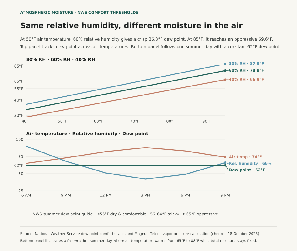
A 60% relative humidity reading feels crisp on a 50°F autumn morning because the dew point sits at 36.3°F, while that same 60% relative humidity feels sticky and oppressive on an 85°F summer afternoon because the dew point reaches 69.6°F. As the National Weather Service (NWS) explains, relative humidity measures how close the air is to saturation at its current temperature, whereas the dew point tracks the temperature at which the water vapor actually present in the air would condense into liquid.

When you check a weather forecast before a run, a commute, or an outdoor shoot, relative humidity alone can point you in the wrong direction. Because warm air can hold substantially more water vapor than cold air before reaching saturation, relative humidity falls every afternoon as the sun heats the ground and rises every night as the air cools - even when the total moisture in the air mass has not changed. Dew point removes that moving temperature denominator and gives you a direct scale for how muggy the air will feel against your skin.

Two-panel chart showing how 60 percent relative humidity corresponds to a 36.3 degree Fahrenheit dew point at 50 degrees air temperature versus a 69.6 degree dew point at 85 degrees air temperature, and how a constant 62 degree dew point causes relative humidity to fall from 90 percent at dawn to 42 percent at 3 PM.
Panel A plots calculated dew point against air temperature along constant relative-humidity curves (40%, 60%, and 80% RH) using the Magnus–Tetens relation across National Weather Service summer comfort thresholds. Panel B shows an illustrative fair-weather summer day where the dew point stays fixed at 62°F while air temperature warms from 65°F at dawn to 88°F at 3:00 PM, cutting relative humidity from 90% to 42%. Reproducible grid: dew-point-relative-humidity-grid.csv.

Why Afternoon Relative Humidity Falls While Muggy Air Stays Put

The NWS Tampa Bay Weather Forecast Office defines the dew point as the temperature to which air must be cooled, at constant pressure, for water vapor to condense into dew, fog, or cloud droplets (100% relative humidity). Because the dew point cannot exceed the air temperature, a 30°F winter morning with a 30°F dew point has 100% relative humidity. By contrast, an 80°F summer afternoon with a 60°F dew point has 50% relative humidity. Even though the percentage is cut in half, the 80°F afternoon contains roughly three times as much water vapor and feels far more humid outside (NWS La Crosse).

Panel B in the figure above follows an illustrative summer day where no front or sea breeze replaces the air mass. At 6:00 AM, the air temperature is 65°F and the dew point is 62°F, producing 90% relative humidity. By 3:00 PM, solar heating pushes the air temperature to 88°F while the dew point remains 62°F. Relative humidity drops from 90% to 42% solely because 88°F air has a much higher moisture ceiling. Your body cools itself by evaporating perspiration from the skin, and the rate of evaporation depends on how much moisture is already in the air. Because that 62°F moisture load never left, sweat evaporates slowly and the afternoon feels warm and sticky despite the 42% relative humidity readout.

Reading the National Weather Service Dew Point Comfort Scale

Forecasters at NWS La Crosse and NWS Tampa Bay group summer dew points into three main comfort bands: 55°F or lower feels dry and comfortable, 56°F to 64°F feels noticeably sticky with muggy evenings, and 65°F or higher indicates heavy atmospheric moisture that feels oppressive. The table below pairs those thresholds with calculated dew points across air temperatures from 50°F to 90°F:

Calculated dew point temperatures (°F) at 40%, 60%, and 80% relative humidity across air temperatures, paired with National Weather Service summer comfort thresholds (NWS La Crosse and NWS Tampa Bay).
Air Temp (°F) Dew Point at 40% RH Dew Point at 60% RH Dew Point at 80% RH Feel at 60% RH (NWS Summer Scale)
50°F 26.9°F 36.3°F 44.0°F Dry and comfortable (≤55°F dew point)
60°F 35.9°F 45.8°F 53.8°F Dry and comfortable (≤55°F dew point)
70°F 44.9°F 55.3°F 63.6°F Threshold of sticky / muggy evenings (55–65°F)
75°F 49.4°F 60.1°F 68.5°F Noticeably sticky; muggy in the evening (55–65°F)
80°F 53.9°F 64.8°F 73.4°F Upper edge of sticky, approaching oppressive (65°F)
85°F 58.4°F 69.6°F 78.3°F Oppressive moisture in the air (≥65°F dew point)
90°F 62.9°F 74.3°F 83.2°F Heavily oppressive; high heat-stress risk (≥65°F)

Where Relative Humidity Still Answers the Right Question

Dew point is the better number for human comfort outdoors, but relative humidity remains the right measure when the question is how fast moisture leaves wood, soil, or foliage at the current temperature. Fire-weather forecasters watch afternoon relative humidity fall below 20% to 30% because dead brush and forest fuels dry out in proportion to the vapor deficit at that hour's air temperature. The same physics explains why indoor air feels parched in January: when outdoor air with a 15°F dew point (and 80% outdoor relative humidity) is drawn inside and heated to 70°F without a humidifier, its relative humidity drops below 15%, pulling moisture from wood floors and skin.

When comparing seasonal climates across cities (see What Are Climate Normals? and Hottest Day on Record vs. Average Summer), looking at temperature and dew point together separates dry desert heat from Gulf Coast humidity. In NWS Tampa Bay's hourly station archive back to 1948, for example, Tampa recorded a peak dew point of 86°F on August 6, 2000, and experienced seven consecutive days with dew points at or above 75°F from August 5–11, 2024 - conditions where nighttime lows cannot cool below the dew point.

Eranorms puts local weather observations into historical context across decades of station records, daily high-low timelines, and upper-air temperature and dewpoint soundings. Open Eranorms in your browser, Download Eranorms for iPhone, or Get Eranorms on Android.
048 / 53

Drought History by State, 2000–2026: Where It Stays and When It Spreads

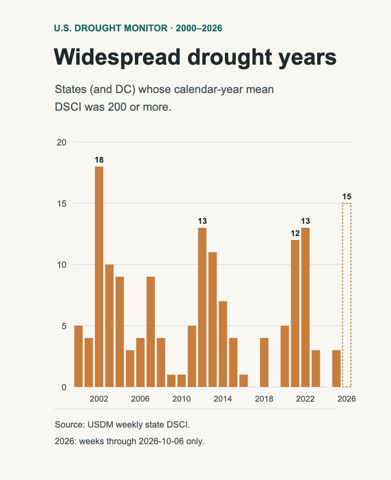
Since 2000, drought in the United States has had a clear home: the Southwest. Arizona, New Mexico, Nevada and Utah averaged a Drought Severity and Coverage Index (DSCI) between 170 and 189 from 2000 through 2025. New York, Pennsylvania and Ohio averaged under 30. But drought also travels. In 2002, 2012, 2021 and 2022, at least a dozen states averaged a DSCI of 200 or more for the year, and 2026 has already pushed drought across the Southeast.

This page uses the U.S. Drought Monitor's weekly record for every state, 4 January 2000 to 6 October 2026, to show where drought tends to stay, when it spreads, and how to read your own state's row.

What the index measures

The Drought Monitor map sorts land into five categories, from D0 (abnormally dry) to D4 (exceptional drought). The DSCI turns a week's map into one number per state: the percentage of the state in D0, plus twice the percentage in D1, three times D2, four times D3 and five times D4 (National Drought Mitigation Center, DSCI). It runs from 0, when no part of the state is even abnormally dry, to 500, when the whole state is in exceptional drought.

A DSCI of 200 can mean all of a state in moderate drought (D1), or about half of it in severe-to-extreme drought with the rest normal. It measures how much of the state is in drought and how bad that drought is, together. The Drought Monitor itself blends rainfall, soil moisture, streamflow and other indicators with expert judgement; the DSCI is a summary of that map, not a rain gauge reading. The NDMC describes it as experimental and says best practices for using it over time are still evolving.

Every state, every month since 2000

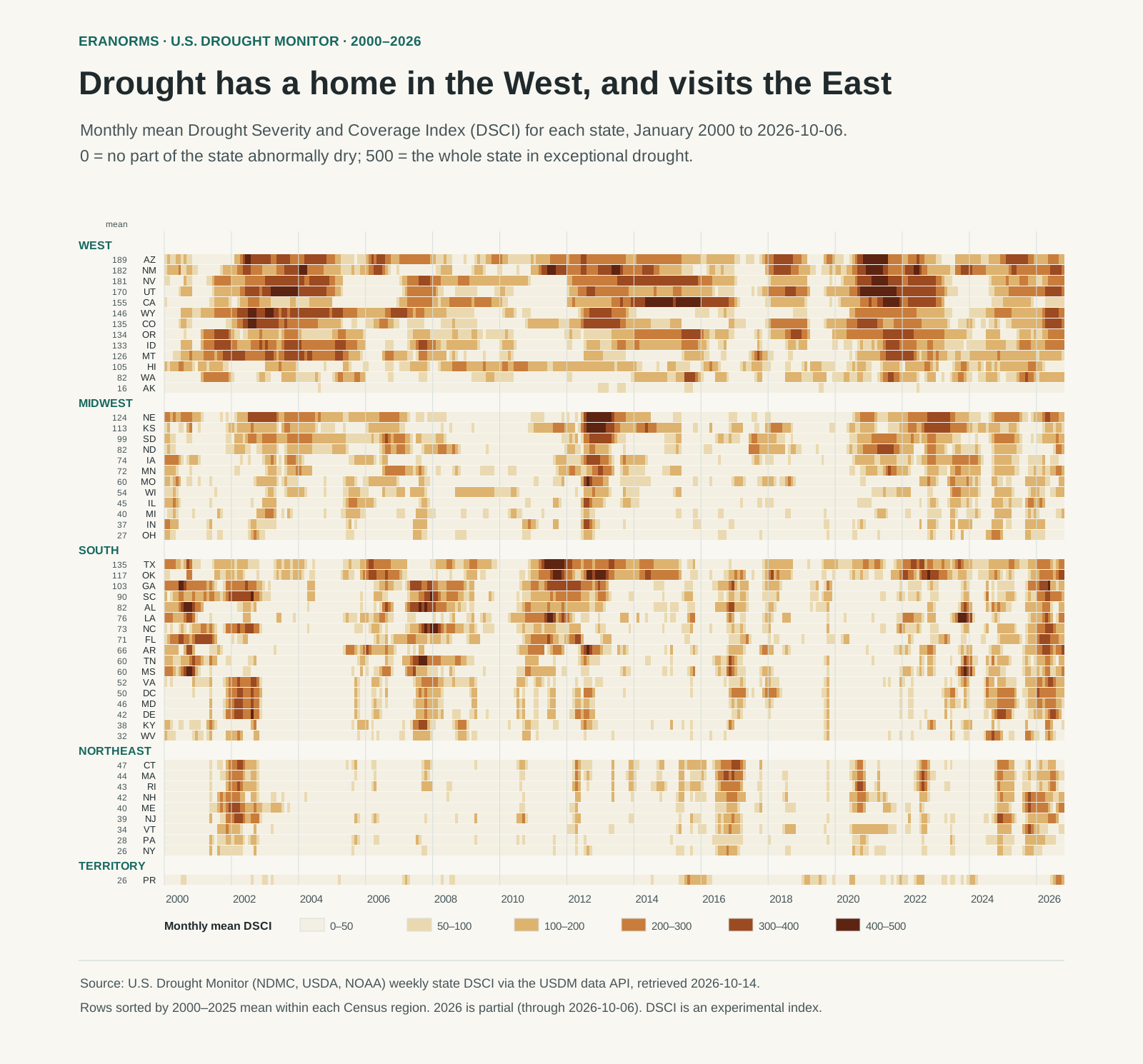
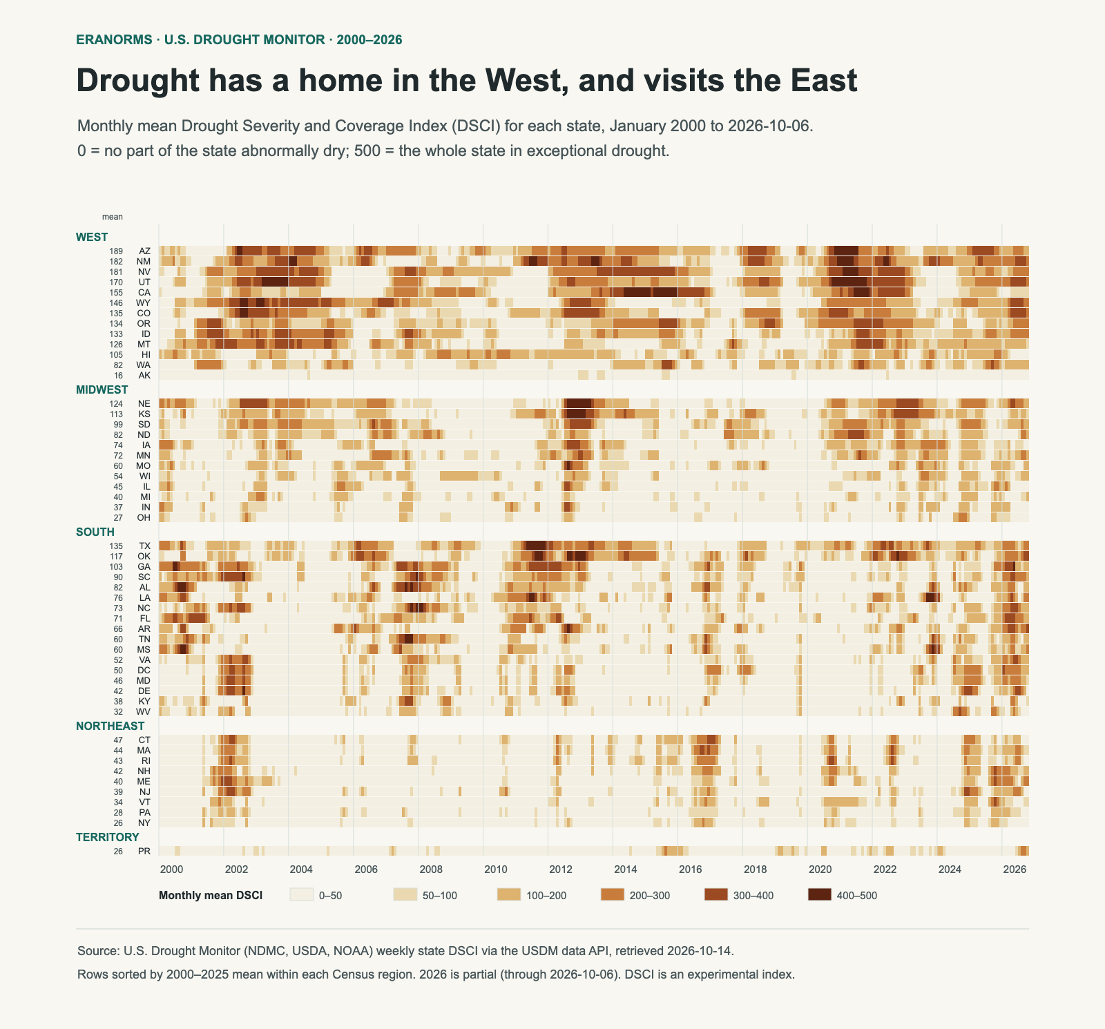
Heatmap of monthly mean drought index for 50 states, DC and Puerto Rico from 2000 to 2026, grouped by region. Western rows are dark for long stretches; Midwest rows darken sharply in 2012; Southern and Northeastern rows are mostly pale with short dark episodes, and many Southern rows darken in 2026.
Each row is a state; each thin column is one month's average of the weekly DSCI. Darker means more of the state in worse drought. Rows are grouped by Census region and sorted by their 2000–2025 average (the number beside each code). 2026 runs through the week of 6 October. SVG · monthly values (CSV) · state summary (CSV) · method and source.

Read the West block first. Arizona, New Mexico, Nevada and Utah are dark for long stretches, sometimes for years: 2002–04, 2012–14 and 2020–22. Drought there is often a multi-year state, not a passing event. California's row shows the 2012–16 drought as one long band, with a yearly average above 400 in both 2014 and 2015.

Now look at the Northeast. Its rows are mostly pale, broken by short, sharp episodes: 2002, 2016, 2020 and the last two years. Massachusetts reached 340 in September 2016, a serious drought, but it had eased by spring 2017. A low long-run average doesn't mean a state never gets drought. It means drought there usually comes and goes faster.

Highest and lowest average DSCI, 2000–2025 (complete years)
StateAverage DSCIWeeks at 300 or moreHighest week
Arizona18918%468 (1 December 2020)
New Mexico18322%440 (14 June 2022)
Nevada18125%414 (13 July 2021)
Utah17022%470 (20 July 2021)
California15518%440 (29 July 2014)
Ohio270%298 (24 September 2024)
New York260%229 (18 October 2016)
Alaska160%101 (23 July 2019)

The "weeks at 300 or more" column counts the whole record through October 2026. Texas has the single highest week of any state, 484 on 13 September 2011, during a year that averaged 383. Its long-run average of 135 is lower than the Southwest's because Texas swings between deep drought and long wet spells.

When drought spreads

Bar chart of the number of states with a yearly average drought index of 200 or more: 18 in 2002, 13 in 2012, 12 in 2021, 13 in 2022, near zero in 2017, 2019 and 2024, and 15 so far in partial 2026.
States (and DC) whose calendar-year average DSCI was 200 or more; Puerto Rico excluded. The 2026 bar, outlined, covers January to early October only, so its count can still change. Download the yearly counts and states.

Most years, only a handful of states average 200 or more. Three periods stand out:

  • 2002: 18 states, from the Mountain West to the mid-Atlantic and Maine: the widest spread of any complete year in this record.
  • 2012–13: the Plains and Midwest. Nebraska shows how fast it arrived: its DSCI was 35 in mid-May 2012 and 414 by mid-August, about thirteen weeks later. In the heatmap that's the sudden dark block in the Midwest rows.
  • 2021–22: the interior West, Pacific Northwest and northern Plains, with Utah's 470 in July 2021 among the highest weeks in the record.

2026 is different. Its 15 so far (14 states and DC) lean south and east: Florida, the Carolinas, Georgia, Arkansas, Virginia, Maryland and DC alongside Colorado, Utah and Wyoming. In the week of 28 April 2026, 14 states and DC were at 300 or more at once, the most of any week since 2000. Several Southeastern states have eased since; Georgia was at 120 on 6 October. A partial year can still change, so treat 2026 as a strong spring and summer, not a finished ranking.

Reading your own state

  1. Find your row and its average. The number beside the state code is its 2000–2025 average. Compare a current reading with that, not with another state's.
  2. Look for bands, not specks. A long dark band is a multi-year drought; scattered dark months are short episodes. They call for different planning.
  3. Remember it's statewide. A state average can hide a county in exceptional drought or a wet corner. Small states and DC reach 0 or 500 more easily, because one weather pattern can cover all of them. For local conditions, check the current Drought Monitor map.
  4. Don't read it as rainfall. A wet month can leave a high DSCI if soil and reservoirs are still depleted. For what rain itself looks like through the year, see average rainfall by month.

Method and limits

Weekly state DSCI values come from the Drought Monitor's data service, retrieved 14 October 2026: 1,397 weeks for each of the 50 states, DC and Puerto Rico. Monthly values are plain averages of that month's weekly maps; state averages use complete years, 2000–2025. Census regions group the rows, and DC sits in the South. This page describes the record. It doesn't adjust for changes in how the map has been drawn since 2000, and it makes no claim about causes or future drought.

The U.S. Drought Monitor is jointly produced by the National Drought Mitigation Center at the University of Nebraska–Lincoln, the U.S. Department of Agriculture and the National Oceanic and Atmospheric Administration. In the Eranorms app, a weather station's analysis dashboard includes this weekly DSCI line for the station's state, so you can see statewide drought next to that station's own record.