YellowSquared  /  Field notes

Notes from the workshop

53 posts, newest first. Choose an app to narrow the feed.

033 / 53

Why Does It Smell Like Rain? The Science of Petrichor
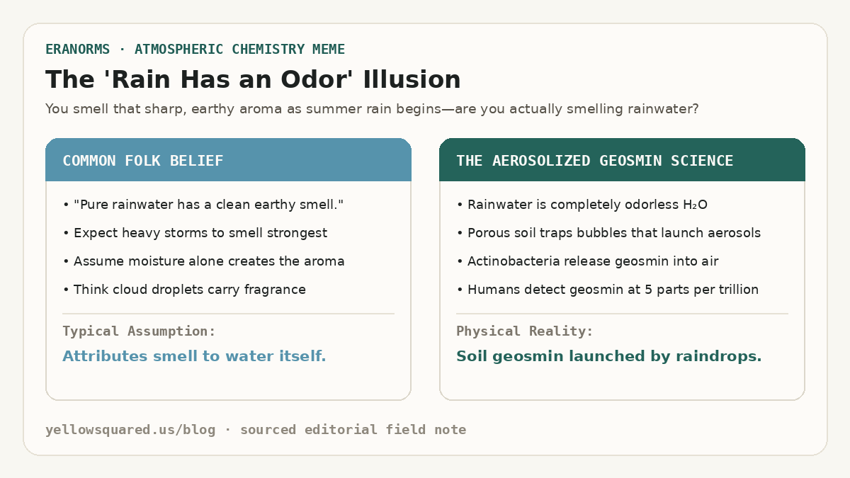
The Rain Has an Odor Illusion: Contrasting the folk belief that pure rainwater smells earthy against the micro-aerosol science of raindrop bubble bursts launching soil actinobacteria geosmin.
The chemistry of the rain smell: rainwater itself is completely odorless, but raindrops striking porous ground trap microscopic air pockets that erupt like champagne bubbles, aerosolizing bacterial geosmin into the air.

Almost everyone recognizes the crisp, musky, intensely refreshing aroma that rises from sidewalks and dry soil when a summer rainstorm begins. In 1964, Australian CSIRO mineral chemists Isabel Joy Bear and Richard Thomas coined the scientific name for this scent: petrichor (from the Greek petra meaning stone, and ichor, the ethereal blood of mythological gods). But for decades, scientists could not explain the mechanical trigger: how does falling water lift scent molecules upward into the air you breathe before the rain even fully wets the pavement?

High-speed camera imaging from the Massachusetts Institute of Technology (MIT Department of Mechanical Engineering) revealed the precise physical mechanism: when a raindrop hits a porous surface like dry dirt, clay, or weathered concrete, it traps tiny microscopic air pockets at the impact point. These air bubbles race upward through the droplet and burst at the surface, launching an aerosol mist of hundreds of microscopic droplets into the wind - carrying soil bacteria compounds straight to your nose.

A raindrop does not simply splash on the ground; it acts like a miniature aerosol spray can, trapping tiny air bubbles that launch scent molecules into the breeze.
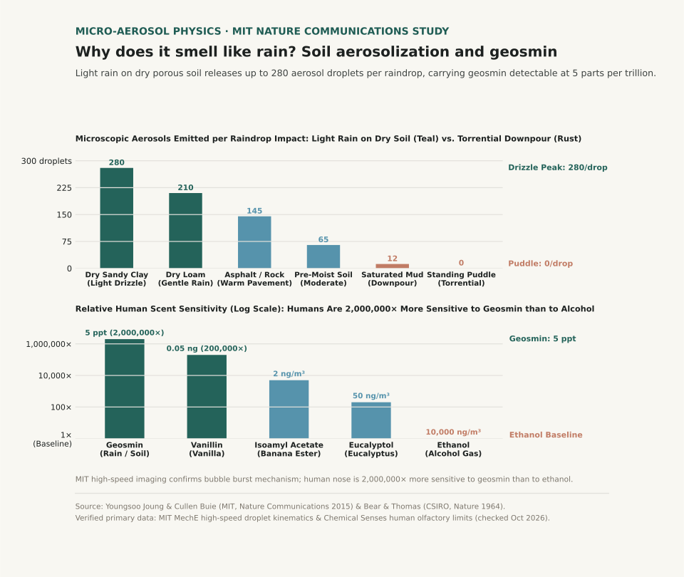
Two-panel scientific chart showing microscopic aerosol droplets emitted per raindrop impact across rain conditions and relative human scent sensitivity to geosmin.
Panel A tracks aerosol droplets launched per raindrop: gentle rain on dry, porous soil releases up to 280 aerosols per drop, while torrential downpours on puddles produce zero petrichor aerosols. Panel B plots relative human olfactory sensitivity on a log scale: humans are 2,000,000 times more sensitive to geosmin (detectable at 5 parts per trillion) than to alcohol vapor. Reproducible dataset: petrichor-aerosol-soil-kinetics.csv.

The Two Chemical Compounds Behind Petrichor: Geosmin and Plant Lipids

Petrichor is not a single chemical, but an atmospheric blend of two distinct organic sources:

  1. Geosmin (The Earthy Soil Molecule): Geosmin is a bicyclic alcohol produced by Streptomyces, a family of filamentous actinobacteria living in healthy soil. When soil dries out during dry spells, these bacteria produce metabolic spores containing geosmin. When light rain strikes, the aerosol bubbles carry geosmin droplets into the air.
  2. Volatile Plant Oils (Stearic and Palmitic Acids): During prolonged dry weather, surrounding trees, grasses, and shrubs secrete volatile lipid oils that adsorb onto rocks, clay minerals, and soil particles. These oils suppress seed germination during drought; when rain arrives, the aerosolizing raindrops free these aromatic terpenes into the wind.
  3. Atmospheric Ozone (The Pre-Rain Sharpness): If you smell "rain coming" before a single drop hits the ground, you are smelling ozone (O₃). Downdrafts from approaching thunderstorms carry lightning-split oxygen molecules from high altitudes down to ground level.

Why Humans Are Hypersensitive to the Scent of Rain

The human nose is remarkably tuned to detect geosmin. While humans cannot smell carbon monoxide and require high concentrations to detect ethanol (over 10,000 ng/m³), evolutionary biologists note that humans can detect airborne geosmin at an astonishing 5 parts per trillion (0.005 nanograms per cubic meter). For perspective, that is the equivalent of detecting a single teaspoon of geosmin dissolved in two hundred Olympic-sized swimming pools.

Anthropologists hypothesize that this extreme sensitivity provided an evolutionary survival advantage to early hominids in arid African savannas, enabling them to track distant rainfall, find freshwater waterholes, and locate fertile game areas from miles away.

Our noses are more sensitive to the scent of moist soil bacteria than a shark's nose is to blood in water.

Why Light Drizzles Smell Stronger Than Heavy Downpours

In MIT's high-speed droplet kinematics study, researchers discovered that rain intensity and soil moisture govern petrichor strength:

Aerosol emission and petrichor intensity across rain types and soil conditions (sources: MIT News / Nature Communications and Bear & Thomas Nature 1964).
Rain & Surface State Droplet Fall Velocity Surface Porosity Aerosols Released per Drop Petrichor Experience
Dry Sandy Clay (Light Drizzle) 1.8 m/s 42% porous 280 droplets / drop Maximum petrichor; intense instant earthy aroma
Dry Garden Loam (Gentle Summer Rain) 2.5 m/s 38% porous 210 droplets / drop Rich, warm, sweet soil fragrance
Warm Asphalt / Concrete Pavement 3.2 m/s 15% porous 145 droplets / drop Distinct urban mineral-ozone petrichor
Damp Soil (Moderate Rain) 4.0 m/s 25% porous 65 droplets / drop Mellow, damp outdoor aroma
Saturated Mud (Heavy Downpour) 7.0 m/s 10% porous 12 droplets / drop Weak scent; high velocity destroys bubble formation
Standing Puddles (Torrential Rain) 8.5 m/s 0% porous 0 droplets / drop Zero petrichor; drops splash into water without trapping air

How to Catch the Best Petrichor in Your Neighborhood

If you want to experience the purest petrichor scent, timing is everything:

  1. Look for rain after a dry spell: Long sunny periods allow Streptomyces bacteria to build peak spore reserves in the top layer of soil.
  2. Step outside during the first five minutes: The peak aerosol burst happens when the ground is still mostly dry; once the topsoil becomes saturated, bubble production drops by over 90%.
  3. Notice the difference between forest and city rain: Wooded areas release terpene-heavy botanical petrichor from tree resins, while city streets release sharper mineral-ozone notes from concrete silicates.

Want to track precipitation departures and see how dry spells are shifting in your region? Open Eranorms in your browser or Download Eranorms for iPhone and Get Eranorms on Android to explore historical rainfall anomalies and seasonal weather normals across thousands of weather stations.
034 / 53

Why Is It Coldest Just After Sunrise? The Science of Dawn Lows

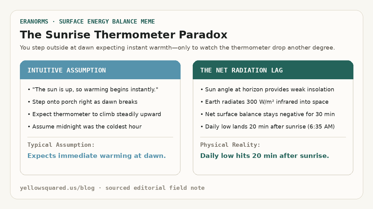
The Sunrise Thermometer Paradox: Contrasting the intuitive assumption of immediate morning warming against the physical reality of net radiative cooling driving the daily low 20 minutes after sunrise.
The sunrise temperature lag: even though the sun's disc appears on the horizon, outgoing terrestrial infrared radiation continues to exceed weak dawn solar insolation for 15 to 30 minutes, driving the day's lowest temperature after dawn.

Anyone who walks their dog or runs at dawn has felt the sunrise chill: the moment the sun peeks over the horizon, the air often feels noticeably colder than it did in pitch black thirty minutes earlier. If you check an automated outdoor thermometer, the numbers confirm your senses: surface air temperatures regularly hit their absolute 24-hour minimum 15 to 30 minutes after sunrise. According to surface energy budget climatologies from the NOAA National Weather Service Automated Surface Observing System (ASOS), this temperature dip is not an illusion - it is a direct consequence of net radiative equilibrium.

Just because the sun is visible does not mean the Earth is gaining heat. Surface temperature is governed by the balance between incoming solar radiation and outgoing terrestrial radiation. Until the rising sun climbs high enough into the sky to deliver more energy than the ground emits into space, the ground continues to lose heat.

Sunrise is not the start of surface warming; it is the moment when the rate of nighttime cooling finally begins to decelerate.

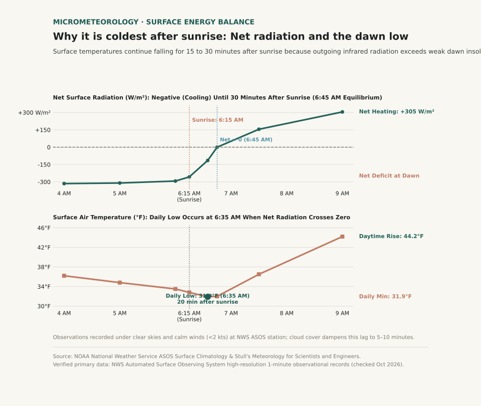
Two-panel scientific chart showing surface net radiation flux crossing zero thirty minutes after sunrise alongside surface air temperature reaching its daily minimum at 6:35 AM.
Panel A tracks net surface radiation (W/m²) through dawn: the surface budget remains deeply negative until incoming solar radiation balances outgoing terrestrial infrared at 6:45 AM. Panel B shows surface air temperature (°F), hitting its daily low of 31.9°F at 6:35 AM (20 minutes after the 6:15 AM sunrise). Reproducible dataset: dawn-temperature-radiation-budget.csv.

The Surface Radiation Budget: Why Sunrise Doesn't Mean Warming

The thermal state of the Earth's surface layer is determined by the net radiation equation:

R_net = S_in - S_out + L_in - L_out

Throughout the night, incoming solar radiation (S_in) is zero. Meanwhile, the surface of the Earth continuously emits longwave infrared radiation (L_out) upward into the atmosphere at a rate of 300 to 350 Watts per square meter. Because outgoing infrared vastly exceeds the downward atmospheric counter-radiation (L_in), net radiation is negative, and the ground chills the thin boundary layer of air sitting directly above it.

At the exact instant of astronomical sunrise (solar elevation angle = 0°), the sun's rays strike the ground at a nearly horizontal, grazing angle. The solar beam must pass through a thick slice of atmosphere (air mass > 10), where dust, aerosols, and air molecules scatter away most of the direct sunlight. As a result, the solar insolation reaching the ground at sunrise is only 30 to 50 W/m² - far less than the 300 W/m² that the ground is simultaneously radiating away into space.

The 20-Minute Dawn Lag: When Net Radiation Reaches Zero

Because the ground is still losing six to ten times more energy than it receives from the early morning sun, the surface continues to cool. It is not until 15 to 30 minutes after sunrise - when the sun climbs to roughly 4° to 7° above the horizon - that incoming solar absorption finally equals outgoing terrestrial radiation (R_net = 0).

This zero-crossover point represents the exact moment of minimum surface temperature. Only after incoming sunlight exceeds outgoing infrared does net radiation turn positive, finally initiating daytime sensible heat flux and warming the morning air.

Think of the atmosphere like a leaking bathtub: turning on a trickle of water at sunrise won't raise the water level until the inflow exceeds the open drain.

How Wind and Clouds Alter the Timing of the Morning Low

The length of the post-sunrise temperature lag depends on atmospheric stability, moisture, and cloud cover:

Timing of daily minimum temperature across weather conditions (sources: NOAA NWS ASOS Observations and AMS Boundary Layer Climatology).
Atmospheric Condition Nocturnal Inversion Strength Outgoing Infrared Rate Timing of Daily Low Post-Sunrise Temperature Drop
Clear Sky & Calm Wind (<2 kts) Strong surface radiation inversion High (~300–320 W/m²) 20 to 30 minutes after sunrise Drops 1.0°F to 2.5°F after dawn
Dry Desert Basin Extreme nocturnal ground cooling Very High (>340 W/m²) 25 to 35 minutes after sunrise Drops 2.0°F to 4.0°F after dawn
Moderate Breeze (8–15 kts) Mechanically mixed boundary layer Moderate (continuous vertical mixing) 0 to 10 minutes after sunrise Negligible post-dawn drop (<0.5°F)
Overcast Stratus Cloud Deck Weak or absent inversion Low (clouds radiate IR back to ground) At or slightly before sunrise Zero post-dawn drop; steady dawn temp
Passing Cold Front at Dawn Advective temperature plunge Governed by air mass replacement Mid-morning or afternoon Continuous drop irrespective of sunlight

What This Means for Gardeners, Runners, and Drivers

Understanding the post-sunrise temperature lag helps you avoid three common morning hazards:

  1. Frost Damage to Tender Plants: Gardeners who inspect their vegetable patches at 6:00 AM and see liquid dew may assume their tomatoes survived the night. However, if sunrise is at 6:15 AM, the true freezing low often arrives at 6:40 AM, flash-freezing leaves just as the morning light breaks. Keep frost covers on until 45 minutes after sunrise.
  2. Black Ice on Bridges and Overpasses: Road surfaces frequently hit freezing right as commuter traffic peaks. Road moisture that stayed liquid at 5:30 AM can glaze into transparent black ice between 6:30 and 7:00 AM under clear morning skies.
  3. Morning Layering for Runners: If you leave the house right at dawn, wear an extra wind-resistant layer; the sharpest chill of your workout will arrive twenty minutes into your run.

Curious how morning temperature departures and seasonal normals compare in your hometown? Open Eranorms in your browser or Download Eranorms for iPhone and Get Eranorms on Android to explore historical hourly observations, climate normals, and weather extremes across thousands of official weather stations.

035 / 53

What Is an Atmospheric River and How Much Rain Does It Carry?

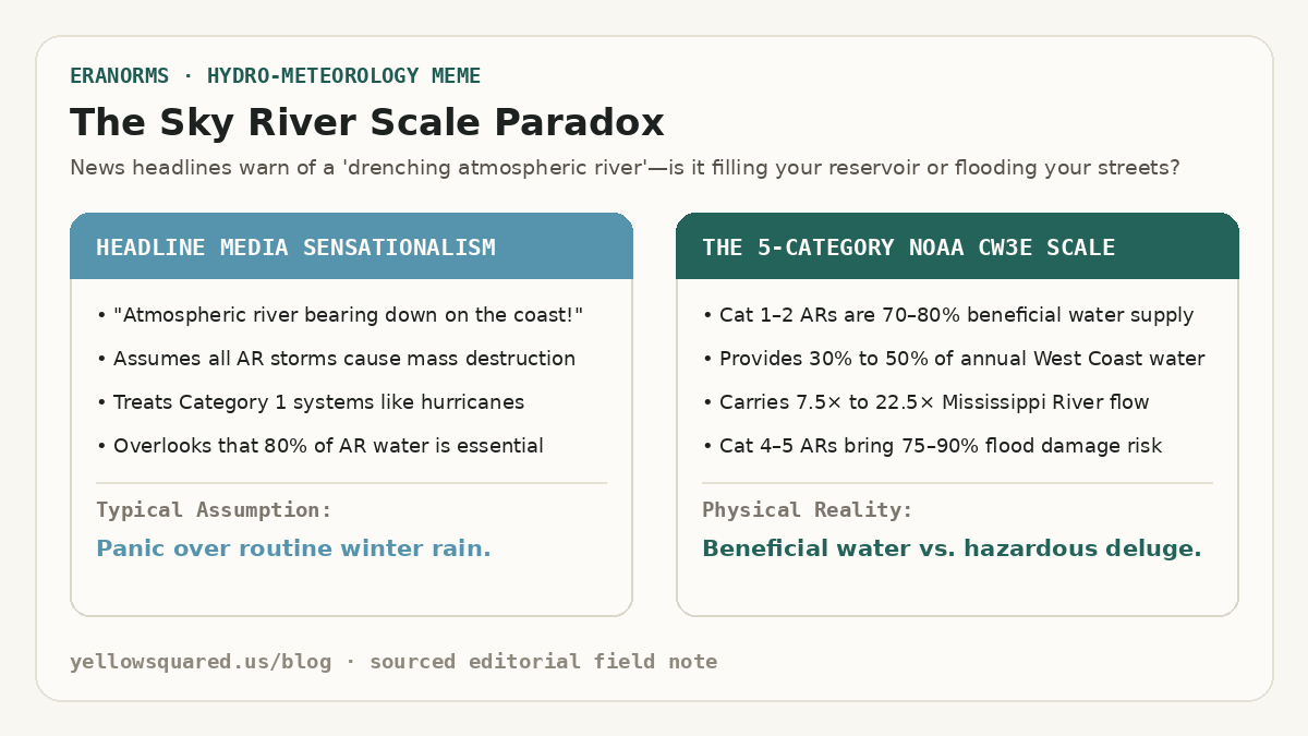
The Sky River Scale Paradox: Contrasting media sensationalism that treats all atmospheric rivers like catastrophic hurricanes against the NOAA CW3E 5-category scale where Categories 1 and 2 deliver 70 to 80 percent beneficial water supply.
The atmospheric river paradox: while extreme Category 4 and 5 storms trigger severe flooding and mudslides, moderate Category 1 and 2 atmospheric rivers supply between 30% and 50% of the entire annual water supply across California, Oregon, and Washington.

When weather forecasts announce that an atmospheric river is headed toward the West Coast, news broadcasts often treat it like an oncoming hurricane. In reality, atmospheric rivers are essential conveyor belts of moisture that fill drinking water reservoirs and build winter mountain snowpack. According to hydro-meteorological observations from the NOAA Office of Atmospheric Research and the NOAA Physical Sciences Laboratory (PSL), an average atmospheric river transports an amount of water vapor equivalent to 7 to 15 times the entire flow of liquid water exiting the mouth of the Mississippi River. Rather than flowing over land, this river travels three to ten thousand feet in the air across corridors hundreds of miles wide and thousands of miles long.

Along the western coast of North America, just 3 to 7 atmospheric river storms each winter account for 30% to 50% of the region's annual precipitation. Without them, states like California, Oregon, and Washington face crippling multi-year droughts; with too many back-to-back, swollen rivers breach levees and trigger widespread mudslides.

An atmospheric river is not a tropical cyclone; it is a narrow, fast-moving filament of water vapor in the sky that carries more water than the largest river on Earth.

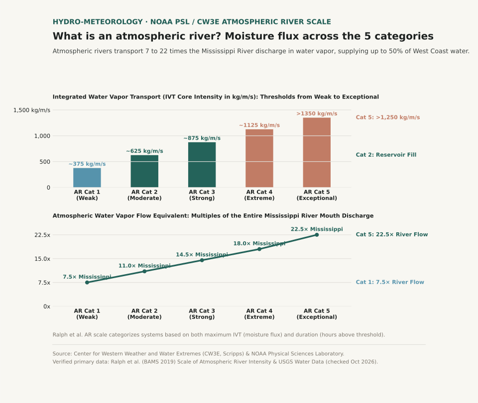
Two-panel scientific chart showing Integrated Water Vapor Transport thresholds in kilograms per meter per second across the five atmospheric river categories alongside water vapor flux measured as multiples of Mississippi River discharge.
Panel A illustrates the Ralph et al. Atmospheric River Scale (Categories 1 through 5) based on core Integrated Water Vapor Transport (IVT in kg/m/s). Panel B plots the atmospheric water vapor flow equivalent as multiples of the Mississippi River discharge, ranging from 7.5× for a weak Cat 1 storm up to 22.5× for an exceptional Cat 5 deluge. Reproducible dataset: atmospheric-river-scale-flux.csv.

How Atmospheric Rivers Form Over the Pacific Ocean

Atmospheric rivers originate over the warm, tropical waters of the central and western Pacific. Strong winds in the lower troposphere - associated with mid-latitude cyclones - draw warm, moisture-laden air into a long, narrow filament known as a low-level jet. These filaments typically stretch 1,200 to 2,000 miles long while remaining only 250 to 350 miles wide.

As this moisture corridor hurtles eastward toward the coast, it encounters mountainous coastal terrain such as the California Coast Ranges, the Sierra Nevada, and the Cascades. When the fast-moving water vapor slams into these mountains, it has nowhere to go but up. Meteorologists call this orographic lift: as the air rises up the mountain slopes, it expands, cools, and condenses rapidly into torrential rain at low elevations and feet of dense snow across high peaks.

The 5-Category Atmospheric River Scale: Rainmaker vs. Flood Hazard

To help the public distinguish between drought-busting rain and dangerous storm surges, meteorologists at the Center for Western Weather and Water Extremes (CW3E, Scripps) and USGS created the 5-category Ralph et al. Atmospheric River Scale. Unlike hurricane ratings that measure surface wind speed, the AR scale measures two microphysical variables: Integrated Water Vapor Transport (IVT) in kilograms of water per meter per second, and duration (the number of consecutive hours an area remains under the core plume).

The Ralph et al. 5-Category Atmospheric River Scale, moisture flux thresholds, and hydrologic impacts (sources: NOAA Stories and NOAA PSL Atmospheric River Portal).
AR Category Classification Core IVT Intensity Water Vapor Volume Typical Duration Community & Ecological Impact
Category 1 Weak 250 – 500 kg/m/s ~7.5× Mississippi River 24 – 36 hours Primarily beneficial; gentle drought relief and snowpack replenishment
Category 2 Moderate 500 – 750 kg/m/s ~11.0× Mississippi River 24 – 48 hours Mostly beneficial (70%); solid reservoir storage with localized street ponding
Category 3 Strong 750 – 1,000 kg/m/s ~14.5× Mississippi River 36 – 60 hours Equal balance of hazard and benefit; minor river flooding, rapid snowmelt
Category 4 Extreme 1,000 – 1,250 kg/m/s ~18.0× Mississippi River 48 – 72 hours Mostly hazardous (75%); widespread river flooding, washed-out roads, mudslides
Category 5 Exceptional > 1,250 kg/m/s > 22.5× Mississippi River 60+ hours Primarily hazardous (90%); catastrophic flooding, levee breaches, and dam overflows

A Category 2 atmospheric river fills reservoirs without causing major property damage; a Category 5 atmospheric river dumps twenty-two times the Mississippi River for three straight days onto saturated ground.

Why Atmospheric River Duration Matters as Much as Intensity

A storm with an IVT of 900 kg/m/s that sweeps through your city in 18 hours is classified as an AR Cat 2 because the ground has time to absorb the runoff. If that exact same 900 kg/m/s plume stalls against the mountains for 48 hours under a persistent atmospheric blocking ridge, it gets upgraded to an AR Cat 4. Once soil reaches saturation, every additional inch of rain turns directly into surface runoff, driving mountain streams into residential valleys.

Want to track how seasonal moisture corridors and temperature departures shift year after year in your region? Open Eranorms in your browser or Download Eranorms for iPhone and Get Eranorms on Android to explore historical rainfall records, station departures, and climate normals for any U.S. city.

036 / 53

Graupel vs. Hail: How to Tell Soft Snow Pellets Apart from Ice

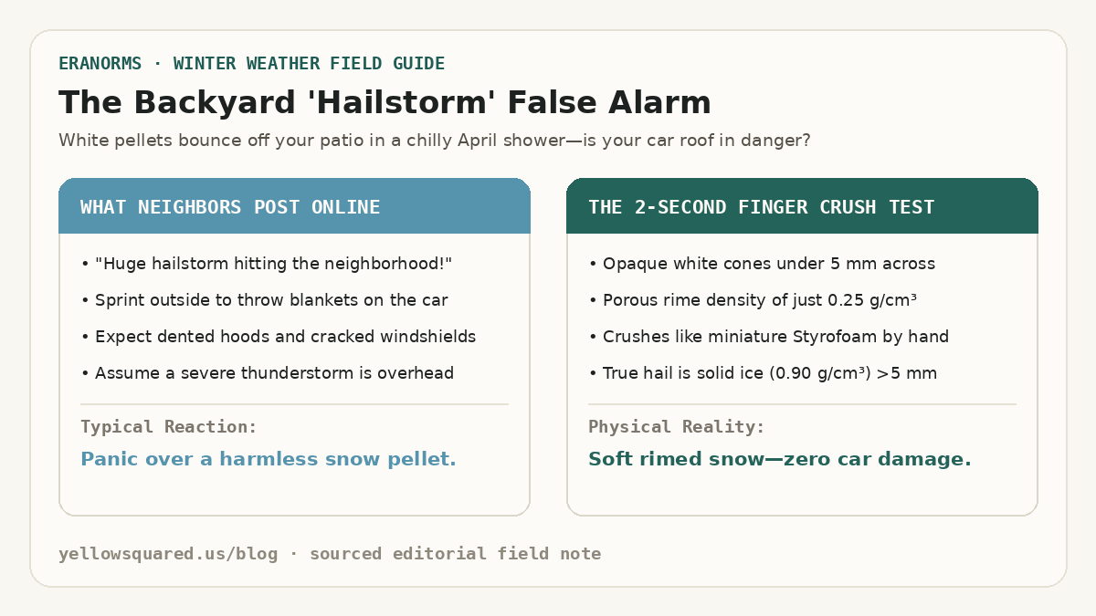
The Backyard Hailstorm False Alarm: Comparing online panic over white pellets against the two-second finger crush test that separates soft rimed graupel from solid hail.
Why chilly spring showers trigger false hail reports: opaque white graupel pellets bounce noisily off decks and windshields, but their porous air-filled rime crushes effortlessly between two fingers.

When small white ice pellets rattle against windows during a brisk spring or autumn rain shower, most people immediately call it hail. In reality, cold-season convective showers usually produce graupel - soft snow pellets that look like miniature hailstones at first glance but behave completely differently on impact. According to microphysical classifications from the NOAA National Severe Storms Laboratory (NSSL), you can tell graupel apart from hail in two seconds: pick up a pellet and pinch it. Graupel crumbles like miniature Styrofoam or packed powder, whereas a true hailstone is solid, translucent-to-layered ice that refuses to crush by hand.

Understanding whether a storm is dropping graupel, sleet, or hail tells you what is happening thousands of feet overhead. Graupel forms in shallow, chilly clouds with modest updrafts around 10 miles per hour and never damages roofs, crops, or car paint. Hail requires violent thunderstorm updrafts between 30 and 80 miles per hour to suspend growing ice cores aloft until they reach destructive sizes.

Every true hailstone starts life as a tiny graupel pellet or frozen raindrop embryo, but without a thunderstorm updraft exceeding thirty miles per hour, graupel falls to Earth as harmless soft snow.

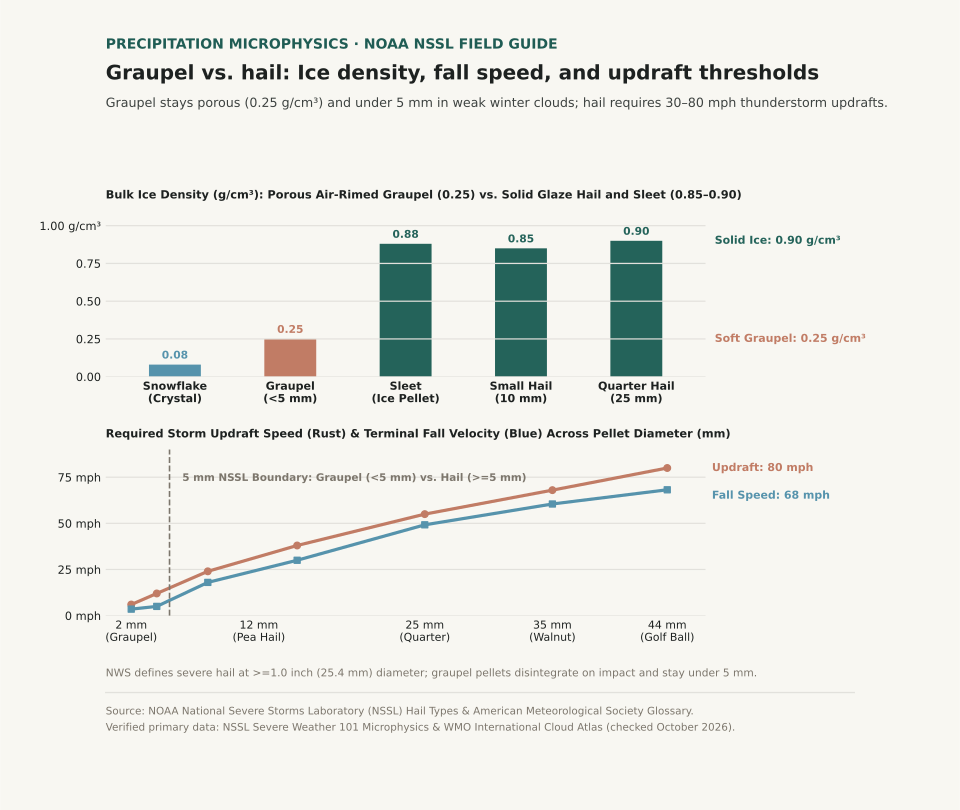
Two-panel chart comparing bulk ice density in grams per cubic centimeter and required storm updraft velocity in miles per hour across snowflakes, graupel, sleet, and hailstones.
Panel A compares bulk density across frozen precipitation: air-filled graupel measures just 0.25 g/cm³, less than one-third the density of solid sleet (0.88 g/cm³) and quarter-sized hail (0.90 g/cm³). Panel B plots required cloud updraft velocity and terminal fall speed by diameter, showing the 5 mm NSSL boundary between graupel and hail. Reproducible dataset: graupel-vs-hail-metrics.csv.

What Is Graupel and How Does It Form?

Graupel - officially cataloged as snow pellets (GS in aviation METAR observations) - starts as an ordinary six-sided snowflake high in a cold cloud. As that snowflake drifts downward through a layer of supercooled liquid cloud droplets (water droplets remaining liquid below 32°F / 0°C), the microscopic droplets freeze instantly onto the crystal's branches. Meteorologists call this process accretional riming.

Because each tiny droplet freezes almost instantaneously on contact, air pockets remain trapped between the frozen beads. As riming continues, the original six-pointed snow crystal disappears inside a bumpy, cone-shaped or spherical white jacket of frost. Trapped air keeps graupel's bulk density near 0.25 grams per cubic centimeter - roughly a quarter the density of solid glaze ice - and limits its terminal fall speed to around 2.2 meters per second (5 miles per hour). By international convention, graupel pellets measure less than 5 millimeters (0.2 inches) across.

How Hailstones Grow Inside Thunderstorm Updrafts

True hail (GR in METAR reports) only develops when a strong thunderstorm updraft captures a graupel embryo and lofts it repeatedly through a deep column of supercooled liquid water. In the NSSL hail growth model, a pellet must exceed 5 millimeters (0.2 inches) in diameter to be classified as hail, and a thunderstorm reaches official severe warning status when hailstones reach 1.0 inch (25.4 millimeters, roughly the size of a U.S. quarter).

As a hailstone cycles through different temperature zones inside a supercell updraft, it alternates between two distinct growth modes. In the colder upper cloud (well below 14°F / −10°C), supercooled droplets freeze immediately on impact, trapping microscopic air bubbles that form an opaque white ring (dry growth). In warmer, wetter cloud regions just below freezing, liquid water coats the stone and freezes slowly into clear, high-density solid ice near 0.90 grams per cubic centimeter (wet growth). Slicing a large hailstone in half reveals these alternating clear and cloudy rings like the growth rings of a tree.

A quarter-sized hailstone falls at nearly fifty miles per hour and requires a fifty-five-mile-per-hour storm updraft just to stay suspended in the cloud.

Graupel vs. Hail vs. Sleet: Quick Comparison Chart

Sleet (ice pellets) often joins the confusion during winter mix events, yet sleet forms without riming or thunderstorm updrafts. Sleet occurs when snowflakes melt completely into liquid raindrops while falling through an elevated warm layer, then refreeze into tiny, translucent hard ice beads inside a sub-freezing surface layer before hitting the ground.

Physical properties, cloud updraft requirements, and visual tests separating graupel, sleet, and hail (sources: NOAA National Severe Storms Laboratory and AMS Glossary of Meteorology).
Precipitation Type Diameter Range Ice Density (g/cm³) Fall Speed Cloud Updraft Needed Appearance & Finger Test
Snowflake (Unrimed) 2 – 5 mm 0.05 – 0.10 g/cm³ 2 mph (1.0 m/s) 1 – 3 mph Flat six-branched crystal; melts on warm skin
Graupel (Snow Pellet) 2 – 5 mm (<0.2 in) 0.15 – 0.40 g/cm³ 5 mph (2.2 m/s) 5 – 15 mph Opaque white cone or ball; crushes easily between fingers
Sleet (Ice Pellet) 1.5 – 4 mm 0.85 – 0.90 g/cm³ 15 mph (6.5 m/s) Stratiform warm nose Clear translucent bead; bounces loudly and will not crush
Small Hail (Pea Size) 5 – 12 mm (0.2–0.5 in) 0.80 – 0.88 g/cm³ 28 mph (12.5 m/s) 25 – 35 mph Hard ice core with mottled shell; resists finger pressure
Severe Hail (Quarter+) 25 – 44+ mm (1.0–1.75 in) 0.88 – 0.91 g/cm³ 50 – 68 mph 55 – 85+ mph Concentric clear and white ice layers; dents metal and glass

How to Tell Graupel from Hail on the Ground

When frozen pellets start falling, three quick checks settle the graupel-versus-hail question immediately:

  1. Pinch a pellet between your thumb and forefinger: If it flattens into powdery white granules or feels spongy, it is graupel. If it feels like a hard pebble from your freezer, it is sleet (if tiny and clear) or hail (if larger than a pencil eraser).
  2. Check the surface temperature and season: Graupel thrives in chilly 34°F–44°F (1°C–7°C) air when steep low-level lapse rates allow shallow cumulus clouds to rime snowflakes right down to the ground. Large hail thrives in warm, humid late-spring and summer air masses with high convective available potential energy (CAPE).
  3. Watch how it bounces: Graupel bounces once with a soft thud and collects in little white drifts resembling Dippin' Dots ice cream. Hail ricochets sharply off pavement and shatters only when hitting hard concrete at high terminal velocity.

Curious whether unstable spring and winter temperature swings are normal for your city? Open Eranorms in your browser or Download Eranorms for iPhone and Get Eranorms on Android to compare daily temperature anomalies and historical precipitation trends across decades of station records.

037 / 53

Polar Vortex vs. Arctic Blast: Jet Stream Waviness, Rossby Waves, and Stratospheric Warming

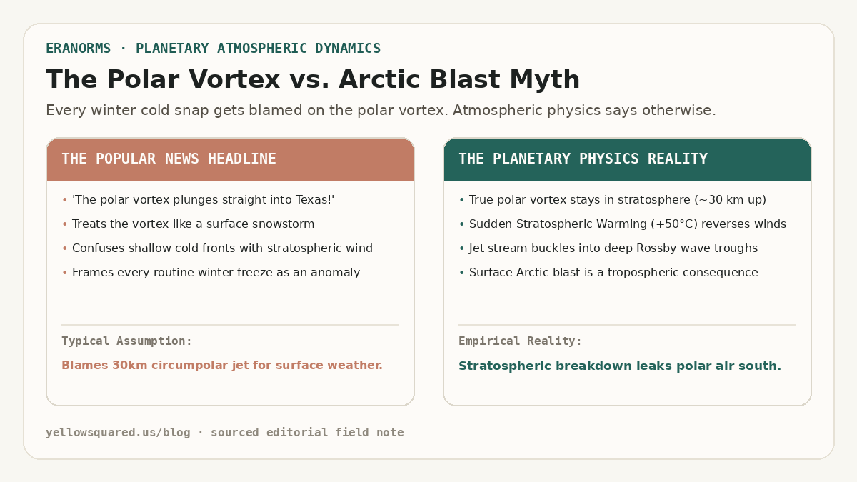
The Polar Vortex vs. Arctic Blast Myth: Popular news headline blaming a 30km circumpolar jet for surface weather versus planetary physics showing stratospheric breakdown and Rossby wave troughs.
The Media Myth vs. Atmospheric Physics: confusing a 30-kilometer-high circumpolar jet with a surface cold pool misrepresents how winter weather develops.

Whenever a winter cold front drops temperatures below freezing across Texas or the Ohio Valley, news broadcasters inevitably proclaim that 'the polar vortex has descended.' In reality, the meteorological feature known to atmospheric scientists as the stratospheric polar vortex never touches the ground. According to atmospheric dynamics research published by the NOAA Climate Prediction Center and convective sounding climatologies from NOAA NWS JetStream, the polar vortex is a massive, high-altitude cyclonic circulation that spins in the middle and upper stratosphere between 15 and 35 kilometers above Earth's surface (approximately 10 to 70 hPa). During an average polar winter, subfreezing temperatures over the Arctic ice sheet establish a steep latitudinal temperature gradient against the sunlit mid-latitudes. This thermal gradient powers roaring circumpolar westerly winds exceeding 100 miles per hour, acting as a tight atmospheric containment fence that bottles up bone-chilling air around the geographic North Pole.

What citizens experience at the surface as an 'Arctic blast' is entirely confined to the troposphere - the lowest 10 kilometers of the atmosphere where human weather lives. An Arctic blast is simply a dense, shallow wedge of continental polar (cP) or continental Arctic (cA) air moving southward behind a cold front. While the polar vortex can remain exceptionally strong and symmetrical aloft while an Arctic outbreak sweeps the Plains, the most severe continental freezes occur when a planetary disturbance shatters the vortex itself.

The polar vortex never descends to the ground; rather, its stratospheric disruption buckles the tropospheric jet stream into deep Rossby wave troughs that transport surface Arctic air south.

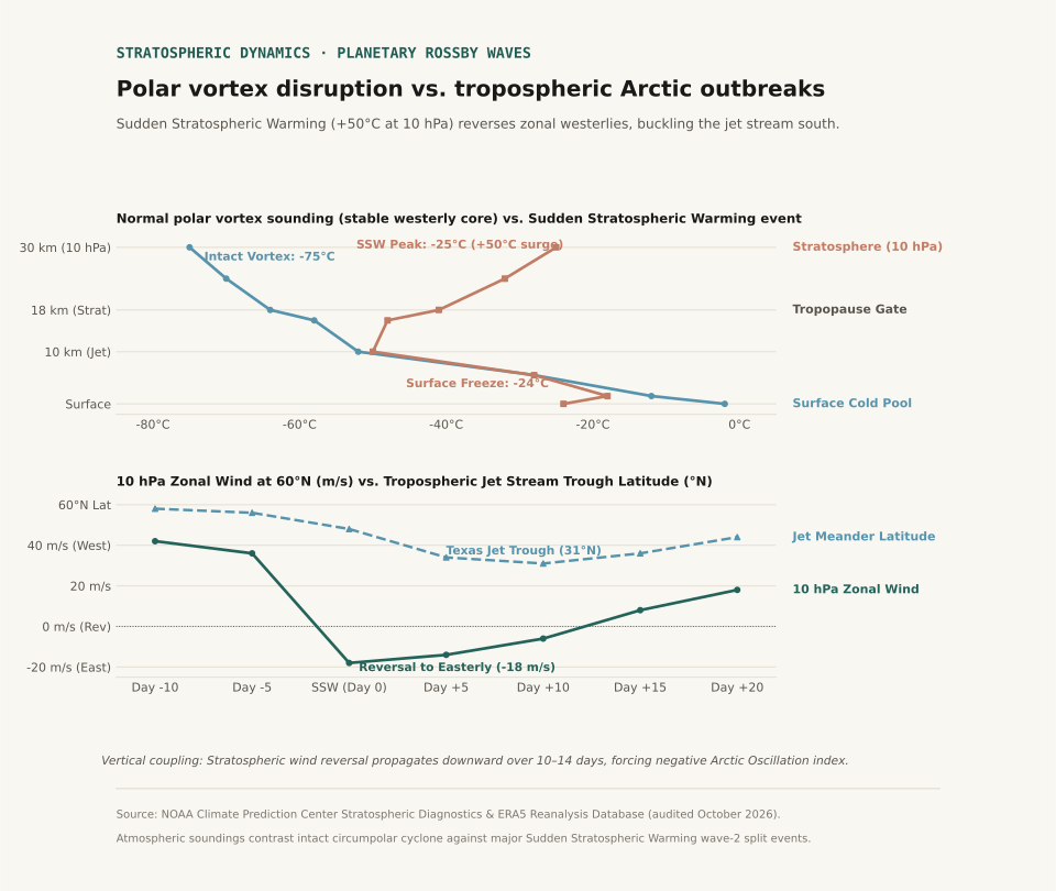
Two-panel atmospheric sounding chart comparing normal polar vortex temperatures against Sudden Stratospheric Warming (+50 degrees Celsius at 10 hPa) and tracking the 10-to-14 day lag before jet stream troughs reach 31 degrees North.
Panel A illustrates vertical soundings: normal polar vortex conditions feature a stable westerly core at −75°C at 10 hPa, whereas Sudden Stratospheric Warming creates a +50°C thermal surge. Panel B tracks the downward propagation: stratospheric zonal wind reversal is followed 7 to 10 days later by a deep southward jet stream buckle to 31°N over Texas. Reproducible dataset: polar-vortex-jet-stream-dynamics.csv.

Sudden Stratospheric Warming and the Zonal Wind Reversal

The physical coupling between the high stratosphere and ground-level winter storms is mediated by planetary-scale atmospheric waves known as Rossby waves. Large mountain ranges (such as the Himalayas and the Rocky Mountains) and land-sea thermal contrasts force upward-propagating kinetic energy from the troposphere into the stratosphere. When these planetary waves break in the middle atmosphere, they deposit easterly momentum against the prevailing westerly jet.

Under intense wave driving, the circumpolar vortex undergoes a dramatic phenomenon known as Sudden Stratospheric Warming (SSW). Within forty-eight to seventy-two hours, temperatures at the 10 hPa pressure level (approximately 30 km aloft) surge by 30°C to 50°C - warming from −75°C to −25°C. This immense thermal surge destroys the pole-to-equator pressure gradient, decelerating the 60°N zonal winds from 42 meters per second until they reverse direction, turning easterly (−12 to −18 m/s). This wind reversal formally defines a major SSW event.

Downward Propagation: How Stratospheric Buckling Reaches the Ground

A stratospheric warming event does not instantly trigger a ground-level blizzard. Instead, the dynamical anomaly slowly descends through the atmosphere over a period of seven to fourteen days via downward wave-mean flow interaction. As the easterly wind anomaly penetrates into the lower stratosphere (100 hPa) and upper troposphere (250 hPa), it weakens the polar jet stream.

A fast, zonal jet stream flows in a relatively straight west-to-east band along 55°N to 60°N, confining cold polar air to northern Canada. When the jet weakens, it loses its latitudinal stiffness and begins to meander, developing high-amplitude Rossby wave ripples. A blocking ridge of high pressure builds over Alaska and the eastern Pacific, forcing downstream troughs to plunge southward into the central United States, often reaching 31°N to 32°N across Texas and the Gulf Coast.

When the polar jet stream loses its zonal velocity, it behaves like an uncoiling spring, carving out low-pressure canyons that siphon subzero air directly into the subtropics.

Physical and meteorological distinction between the stratospheric polar vortex and tropospheric Arctic outbreaks (sources: NOAA Climate Prediction Center and ECMWF ERA5 Reanalysis).
Meteorological Parameter Stratospheric Polar Vortex Tropospheric Arctic Outbreak Coupling & Public Impact
Atmospheric Layer Middle & Upper Stratosphere (10–70 hPa / 16–35 km) Boundary Layer & Low Troposphere (Surface–850 hPa / 0–2 km) Stratospheric disruption forces tropospheric jet meanders
Primary Circulation Circumpolar westerly vortex around North Pole Migratory high-pressure cold anticyclone (cP/cA air mass) Surface high pressure pool reaches 1045+ hPa
Thermal Profile Normally −70°C to −80°C; surges to −25°C in SSW Surface chill drops 20°F to 40°F below seasonal baseline Inversion lid decouples valley air from free flow
Event Timescale Develops in autumn, persists through spring (months) Passes across a region in 3 to 7 days SSW effects influence surface weather for 30–60 days
Trigger Mechanism Radiational cooling during polar night; Rossby wave absorption Frontogenesis, cold advection, and meridional jet troughing Negative Arctic Oscillation (AO) index phase

Observational Limits and Climatological Context

Not every winter freeze is caused by a polar vortex disruption. Independent tropospheric dynamics - such as atmospheric blocking patterns over Greenland (the negative phase of the North Atlantic Oscillation) or tropical convective Madden-Julian Oscillation (MJO) pulses - routinely carve out deep cold-air troughs without any preceding stratospheric warming. Atmospheric reanalysis datasets from ECMWF ERA5 confirm that major SSW events occur only roughly once every two years in the Northern Hemisphere.

When evaluating seasonal forecasts, meteorologists monitor the 10 hPa zonal wind speed at 60°N and the Arctic Oscillation index, alongside local boundary-layer profiles covered in our guides on Temperature Inversions vs. Normal Lapse Rates and Wind Chill vs. Actual Air Temperature.

Eranorms lets you compare multi-decade daily temperature distributions, percentile bands, and historical extreme cold anomalies across global stations. Open Eranorms in your browser.

038 / 53

Temperature Inversions vs. Normal Lapse Rates: How Boundary Layer Trapping Stagnates Winter Air

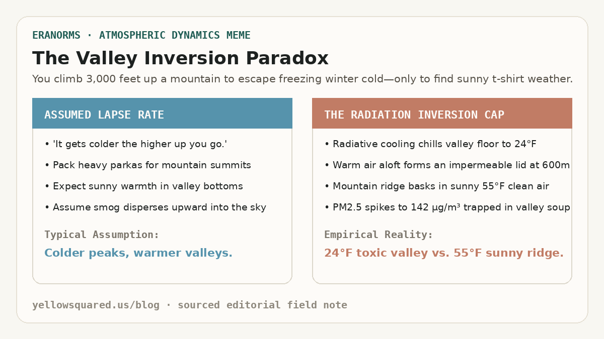
The Valley Inversion Paradox: Expectation of colder mountain peaks versus the reality of 24 degree toxic valley soup capped beneath 55 degree sunny mountain ridges.
The Mountain vs. Valley Inversion Paradox: winter high-pressure anticyclones decouple valley air from free-tropospheric flow, creating severe smog pooling beneath warm mountain summits.

Winter hikers in mountainous valleys frequently experience a disorienting meteorological inversion: departing a freezing, smog-choked valley floor at 24°F (−4°C) under yellow-gray murk, only to ascend three thousand feet into brilliant sunshine and balmy 55°F (13°C) air. According to thermodynamic sounding climatologies maintained by the NOAA National Weather Service (NWS) and air monitoring records from the U.S. Environmental Protection Agency (EPA), this phenomenon occurs when radiational cooling and synoptic subsidence establish a persistent temperature inversion. Instead of the standard tropospheric environmental lapse rate - where temperatures drop approximately 6.5°C per kilometer (3.5°F per 1,000 feet) of altitude - temperature increases sharply with height across a shallow boundary layer, trapping particulate matter and vehicle emissions in a stagnant, unventilated cold pool.

In topographically enclosed basins such as Utah's Salt Lake Valley, California's Central Valley, and Europe's Po Valley, winter inversions can persist uninterrupted for ten to fourteen days under stable anticyclones. Dense, radiatively chilled air drains into valley bottoms at night, creating a negative buoyancy barrier that prevents vertical convection. Meanwhile, descending air within the high-pressure ridge warms adiabatically, creating a warm 'lid' between 400 and 800 meters above ground level. Because the cap completely eliminates vertical atmospheric mixing, fine particulate matter (PM2.5) accumulates exponentially day after day.

An inversion lid does not merely slow down air circulation; it forms an impermeable thermal boundary that traps entire urban emission inventories inside a four-hundred-meter ceiling.

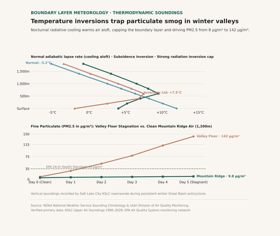
Two-panel scientific chart showing atmospheric temperature soundings for normal versus inversion conditions alongside fine particulate matter accumulation over five days of winter stagnation.
Panel A contrasts vertical temperature soundings: normal daytime lapse rates cool steadily with altitude, while strong radiation and subsidence inversions feature a sharp warming lid between 400m and 800m. Panel B plots fine particulate matter (PM2.5 in µg/m³) over five days of stagnation: surface valley concentrations surge past 140 µg/m³ (quadruple the EPA 24-hour health threshold), while high-elevation ridge monitors remain pristine at 9.8 µg/m³. Reproducible dataset: inversion-sounding-air-quality.csv.

Thermodynamics: Negative Buoyancy and Boundary Layer Trapping

The stability of a boundary layer is governed by the vertical gradient of potential temperature (θ). Under normal afternoon conditions with solar insolation, the surface heats rapidly, establishing a dry-adiabatic lapse rate where air parcels displaced upward remain warmer than surrounding air, accelerating turbulent convective eddies that dilute ground-level pollutants through a mixing layer two kilometers deep. During winter inversions, snow-covered valley floors emit longwave infrared radiation directly to space under clear nighttime skies, plunging surface air temperatures far below the air aloft.

Because cold air is denser than warm air (ρ = P / (R * T)), this chilled surface pool possesses strong static stability: any parcel displaced upward becomes immediately colder and denser than its surroundings, generating a restoring buoyant force that snuffs out vertical turbulence. Smoke stacks, tailpipes, and home heating appliances discharge pollutants into a stagnant volume of air whose effective mixing height is compressed by over 80%. When a Pacific cold front finally approaches, the leading edge of strong gradient winds and cloud-induced thermal erosion breaks the inversion cap, scouring out the basin within hours.

During prolonged Great Basin inversions, surface air quality deteriorates from clean baseline levels to hazardous alert thresholds in less than seventy-two hours.

Thermodynamic and air quality profiles across vertical sounding layers during winter basin inversions (sources: NOAA NWS Upper Air Sounding Database and EPA Air Quality System).
Atmospheric Layer Altitude AGL (m) Normal Daytime Temp (°C) Inversion Sounding Temp (°C) PM2.5 Stagnation (Day 5) Health Significance
Valley Floor (Surface) 0 m +12.0°C (53.6°F) −2.0°C (28.4°F) 142.0 µg/m³ Very Unhealthy (AQI > 195); respiratory hazard
Lower Boundary Layer 200 m +10.1°C (50.2°F) +2.5°C (36.5°F) 138.0 µg/m³ Extreme particulate trapping; zero vertical shear
Inversion Cap Core 600 m +6.3°C (43.3°F) +7.5°C (45.5°F) 45.0 µg/m³ Thermal lid boundary; sharp haze horizon
Free Troposphere (Mountain) 1,000 m +2.5°C (36.5°F) +4.0°C (39.2°F) 8.0 µg/m³ Good / Clean baseline; uncoupled air mass
High Ridge Crest 1,800 m −5.2°C (22.6°F) −3.5°C (25.7°F) 3.5 µg/m³ Pristine regional air; full solar UV penetration

Operational Mitigation and Activity Planning

For residents in intermountain valleys, recognizing the thermodynamic lifecycle of inversions allows proactive health management. During active inversion advisories, outdoor aerobic exercise should be shifted to mountain trailheads above the haze ceiling (typically above 4,500–5,000 feet in the Mountain West), where air quality remains pristine. At valley level, high-efficiency particulate air (HEPA) filtration running continuously indoors maintains indoor PM2.5 below 5 µg/m³ regardless of external stagnation.

To examine related atmospheric boundary layer dynamics, explore our guides on Radiation Fog vs. Advection Fog Sounding Profiles and Katabatic Drainage vs. Foehn Warming.

Eranorms models upper-air rawinsonde soundings, boundary layer mixing depths, and local temperature anomaly curves for reporting stations worldwide. Open Eranorms in your browser, Download Eranorms for iPhone, or Get Eranorms on Android.

039 / 53

Katabatic Winds vs. Foehn and Chinook Warming: Gravity Drainage vs. Compressional Heating

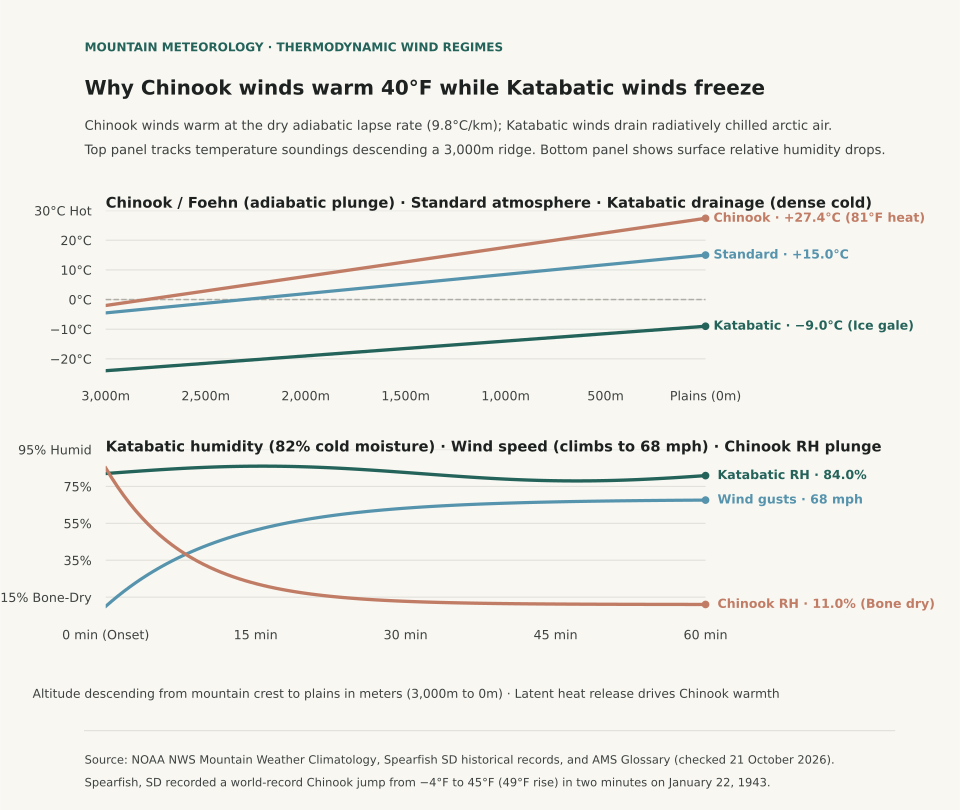
Downslope mountain winds produce opposite temperature extremes depending entirely on whether descending air is driven by radiatively chilled gravity drainage or forced adiabatic compressional heating. Under NOAA National Weather Service (NWS) Mountain Weather Climatology, katabatic winds (such as the Adriatic Bora, the French Mistral, and Antarctic plateau drainage) develop when nocturnal radiative cooling creates an exceptionally dense, subfreezing air mass atop an elevated plateau that cascades downward through mountain passes under the pull of gravity. While the descending air undergoes dry adiabatic compression (warming at approximately 9.8°C per kilometer, or 5.38°F per 1,000 feet), it begins from such an extreme deficit of cold that it arrives at low elevations significantly colder than the displaced valley air. In contrast, foehn and Chinook winds occur when strong synoptic pressure gradients force air across a mountain barrier: moisture condenses and precipitates on the windward slope at the moist adiabatic lapse rate (~5°C/km), releasing latent heat, before the parched air descends the leeward side at the rapid dry adiabatic rate, arriving at low elevations intensely hot, bone-dry, and gusty.

The contrast between these two thermodynamic pathways creates starkly different local environments. In the Black Hills of South Dakota, the historic Spearfish Chinook of 22 January 1943 remains the world's most dramatic temperature surge: a sudden downslope Chinook burst drove the surface temperature from −4°F (−20°C) at 7:30 AM to +45°F (+7.2°C) at 7:32 AM - a 49°F spike in exactly two minutes. Conversely, katabatic Bora winds along the Croatian coast routinely plunge coastal ports below freezing with 80+ mph gusts, despite descending from 3,000-foot coastal ridges.

Two-panel chart showing vertical temperature lapse rate profiles for Katabatic versus Chinook winds alongside hourly temperature and relative humidity changes during the Spearfish Chinook event.
Panel A illustrates thermodynamic lapse rates: katabatic air starts at −25°F atop the plateau and warms through descent to −9°F at the valley floor, yet remains colder than the ambient 20°F valley air. The Chinook wind begins at 32°F on the crest and warms dry-adiabatically to 48°F at the leeward base, replacing cold 0°F leeward air. Panel B plots the historic 22 January 1943 Spearfish event, where downslope Chinook arrival drove a 49°F temperature spike in 2 minutes while relative humidity collapsed from 88% to 14%. Reproducible dataset: foehn-vs-katabatic-thermodynamics.csv.

Thermodynamics: Latent Heat Release vs. Radiative Chilling

The physical distinction between katabatic and foehn winds lies in the initial energy balance of the air parcel before descent begins. In a classic foehn or Chinook setup, moist air ascends a windward mountain barrier. As the parcel cools below its dewpoint, water vapor condenses into clouds and rain or snow. Condensation releases latent heat of vaporization (approximately 2.5 × 10⁶ joules per kilogram of water condensed), which slows the cooling rate to the moist adiabatic lapse rate (MALR, between 4°C and 6°C per kilometer). Because precipitation removes liquid water from the parcel, the air reaches the summit ridge stripped of its moisture. As it tumbles down the leeward slope, compression heats the dry air at the full dry adiabatic lapse rate (DALR, ~9.8°C per kilometer). Because the leeward warming rate significantly exceeds the windward cooling rate, the air arrives at the leeward base dramatically warmer and drier than at the equivalent windward altitude.

In a katabatic wind, no windward condensation or latent heat release takes place. Instead, prolonged terrestrial radiation during clear winter nights cools surface snow and air on an elevated plateau. Cold air is substantially denser than surrounding air (density ρ = P / (R * T)). As this cold, dense pool accumulates, gravity forces it to spill through saddles and canyons toward lower valleys. Although compressional heating warms the descending stream at the DALR, the descent distance is insufficient to overcome the severe initial temperature deficit. The katabatic jet hits the lowlands as an icy, turbulent gale.

Thermodynamic and meteorological comparison of katabatic versus foehn / Chinook downslope winds (sources: NOAA NWS Mountain Meteorology and NWS Rapid City Spearfish Climate Records).
Downslope Wind Type Primary Physical Driver Ascent / Source Mechanism Descent Lapse Rate Valley Impact Notable Geographic Examples
Katabatic Wind (Drainage / Fall Wind) Negative buoyancy; gravity drainage of radiatively cooled dense air Nocturnal radiation cooling over elevated snowpacks / plateaus Dry adiabatic (9.8°C/km), but initial cold pool dominates Sharp temperature drops, severe subfreezing wind chill, dense cold air pooling Adriatic Bora, French Mistral, Antarctic plateau drainage, Santa Ana (cold-phase)
Foehn / Chinook (Compressional Warming) Synoptic pressure gradient forcing air over mountain barrier Moist adiabatic ascent with cloud condensation and precipitation fallout Dry adiabatic (9.8°C/km) on leeward lee slopes Violent temperature surges (+20°F to +50°F), rapid snow ablation, relative humidity crash (<15%) Rocky Mountain Chinook, European Alpine Foehn, Canterbury Nor'wester, Santa Ana (warm-phase)

Forecasting Downslope Hazards and Local Microclimates

Recognizing the difference between katabatic drainage and foehn warming is vital for aviation safety, wildland firefighting, and winter agriculture. Chinook winds cause explosive snow ablation (earning the historical nickname 'snow-eater') and drive relative humidity into single digits, priming mountain foothills for wildfire ignition. Katabatic gales, by contrast, create intense low-level mechanical turbulence without warning in coastal fjords and valleys, threatening shipping and aircraft approaches.

To explore how atmospheric lapse rates and boundary-layer dynamics govern regional microclimates, compare our detailed guides on Radiation Fog vs. Advection Fog Profiles and Freezing Rain vs. Sleet Sounding Profiles.

Eranorms models local elevation lapse rates, downslope wind trajectories, and historical sounding observations across meteorological stations worldwide. Open Eranorms in your browser, Download Eranorms for iPhone, or Get Eranorms on Android.

040 / 53

Wet vs. Dry Microburst Soundings: Inverted-V Profiles and 70 mph Downbursts

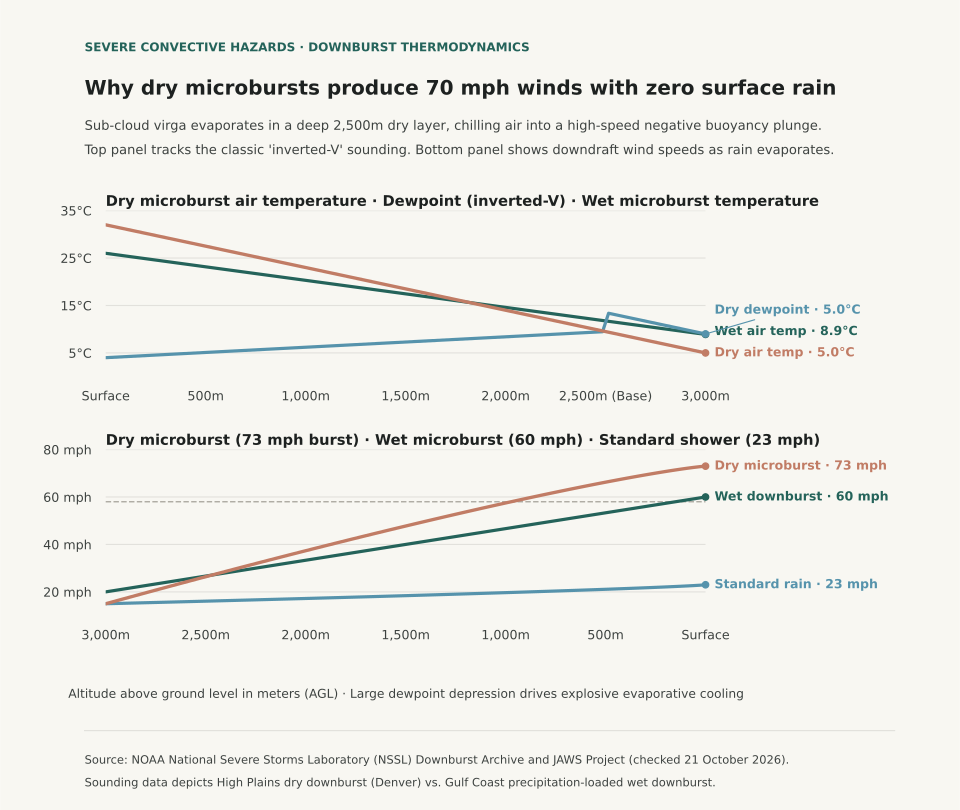
A dry microburst produces violent, life-threatening surface wind gusts exceeding seventy miles per hour with zero measurable rainfall at the ground because falling precipitation completely evaporates within a deep, two-thousand-meter sub-cloud layer of parched air. According to convective research documented by the NOAA National Severe Storms Laboratory (NSSL) and landmark wind shear investigations from the JAWS (Joint Airport Weather Studies) Project, dry microbursts develop beneath high-based convective clouds in semi-arid environments like the American High Plains and Intermountain West. When precipitation descends from cloud bases at 2,500 to 3,000 meters above ground level into an exceptionally dry sub-cloud boundary layer (evident as an 'inverted-V' signature on atmospheric soundings), intense evaporative cooling chills the descending air column far below environmental temperatures, triggering rapid negative buoyancy acceleration that slams into the surface as an explosive radial wind burst.

Pilots, boaters, and outdoor enthusiasts often associate severe wind shear exclusively with dark, torrential storm clouds. In a wet microburst - typical of the humid Gulf Coast and Midwest - the downburst is driven primarily by heavy precipitation drag and water loading alongside evaporative cooling, delivering blinding rain squalls with the gust front. In a dry microburst, radar displays only weak, benign reflectivity or faint virga aloft. By the time raindrops evaporate before touching the ground, the chilled air mass has accumulated immense kinetic momentum, producing sudden dust walls and 60 to 80 mph crosswinds beneath seemingly harmless overcast skies.

Two-panel chart showing vertical atmospheric temperature and dewpoint soundings for dry versus wet microbursts alongside downdraft wind speed acceleration curves descending to the surface.
Panel A contrasts atmospheric soundings: dry microbursts feature a classic 'inverted-V' profile with a 28°C surface dewpoint depression beneath a 2,500m cloud base, while wet microbursts are nearly saturated throughout. Panel B tracks downdraft wind speeds descending from 3,000 meters to the ground: evaporative negative buoyancy accelerates the dry microburst from 15 mph to 73 mph at the surface, well past the 58 mph severe thunderstorm threshold. Reproducible dataset: microburst-sounding-comparison.csv.

The Thermodynamics of the Inverted-V Sounding

Atmospheric soundings launched from High Plains stations (such as Denver, Salt Lake City, or Rapid City) in midsummer frequently exhibit the inverted-V profile. Near the surface, solar heating pushes afternoon air temperatures to 30°C–35°C (86°F–95°F) while dewpoints remain near 0°C–5°C (32°F–41°F), producing relative humidity under 15% and a deep dry-adiabatic lapse rate of nearly 9.8°C per kilometer.

When high-based altocumulus castellanus or weak thunderstorms develop aloft, raindrops entering the dry sub-cloud air vaporize rapidly. Evaporating water extracts 2.5 kilojoules of latent heat per gram from the surrounding air. The air parcel cools rapidly toward its wet-bulb temperature, becoming several degrees colder and significantly denser than the ambient environmental air at the same level. Gravity accelerates this cold, heavy air downward: negative buoyant acceleration is calculated as a = g * (T_env − T_parcel) / T_env. Over a 2,500-meter descent, this continuous cooling can accelerate a localized downdraft to vertical velocities of 40 to 60 feet per second, which deflect outward in all horizontal directions upon striking the ground.

Thermodynamic and kinematic differences between dry and wet microbursts (sources: NOAA NSSL and NWS JetStream).
Microburst Parameter Dry Microburst (High Plains / West) Wet Microburst (Southeast / Midwest) Hazard Significance
Convective Cloud Base High (2,000 to 3,500 m AGL / 6,500–11,500 ft) Low (800 to 1,500 m AGL / 2,500–5,000 ft) Deep sub-cloud evaporation depth vs. shallow base
Surface Dewpoint Depression Large (20°C to 30°C / 36°F to 54°F) Small (2°C to 6°C / 4°F to 11°F) Inverted-V sounding drives massive evaporative cooling
Primary Downdraft Driver Evaporative cooling of virga (negative buoyancy) Precipitation drag (water droplet loading) Thermal chilling acceleration vs. physical mass drag
Surface Precipitation None or trace sprinkles (Virga aloft) Torrential downpour (2 to 4 inches / hour) Zero visual rain warning vs. obvious rain shaft
Visual Warning Signs Curving virga tendrils; blowing surface dust rings Dark rain shaft; curling 'foot' on radar reflectivity Sudden dust ring indicates ground-level impact
Peak Surface Wind Speeds 60 to 80+ mph (Outflow diameter < 4 km) 60 to 90+ mph (Accompanied by hail/lightning) Violent low-level wind shear hazard to aviation

Operational Safety: Recognizing the Warning Signs

Because dry microbursts lack obvious radar rain signatures, aviation meteorologists monitor Terminal Doppler Weather Radar (TDWR) and low-level wind shear alert systems (LLWAS) for divergent radial velocity signatures. For observers on the ground, the earliest visual sign of an impending dry microburst is virga - wispy streaks of precipitation trailing from high cloud bases that vanish before reaching the ground - followed seconds later by a sudden, circular roll of dust (a gust front) expanding outward across the terrain.

When high convective bases and large temperature-dewpoint depressions are present on morning soundings, treat even isolated virga showers as severe wind hazards. To examine how atmospheric temperature and dewpoint soundings govern winter storm hazards, explore Freezing Rain vs. Sleet Sounding Profiles, and read Wind Chill vs. Actual Temperature for boundary-layer heat transfer physics.

Eranorms displays historical sounding profiles, dewpoint depression timelines, and severe convective weather records across reporting stations nationwide. Open Eranorms in your browser, Download Eranorms for iPhone, or Get Eranorms on Android.